2 + 3[1] 54/5[1] 0.8sqrt(23)[1] 4.795832Here we will provide a gentle introduction to computing in R. One of the great things about R as a programming language is the number of free online resources. This chapter will have some basics to get you started, along with lots of places to learn more and to find help.
Getting your computing environment set up and working is the most important task in the first week of this class!
Installing R and RStudio is quite straightforward. One advantage of using RStudio is that you do not need to be connected to the internet, unlike Jupyter.
To set this up the order is quite important.
We first install R, and download it at this link
Then, when that is completed, install RStudio, which can be downloaded at this link
This series of YouTube videos are very clear on how this works and consider Mac Windows and Linux computers. If anyone is using a Chromebook you will have to use the alternative Jupyter setup described below.
If you have previously used R with Jupyter and would prefer to use that format again, that is completely fine.
One advantage is that you do not need to install any software to use Jupyter, and can do it all in the browser.
You can access Jupyter at https://sfu.syzygy.ca/.
For this class it will be sufficient but if you will be using R for further projects, I would recommend using RStudio.
When you first open Jupyter it will give you a slightly different setup to RStudio.
After a few moments this will bring you to a page which looks like the below screenshot, without any folders on the left.
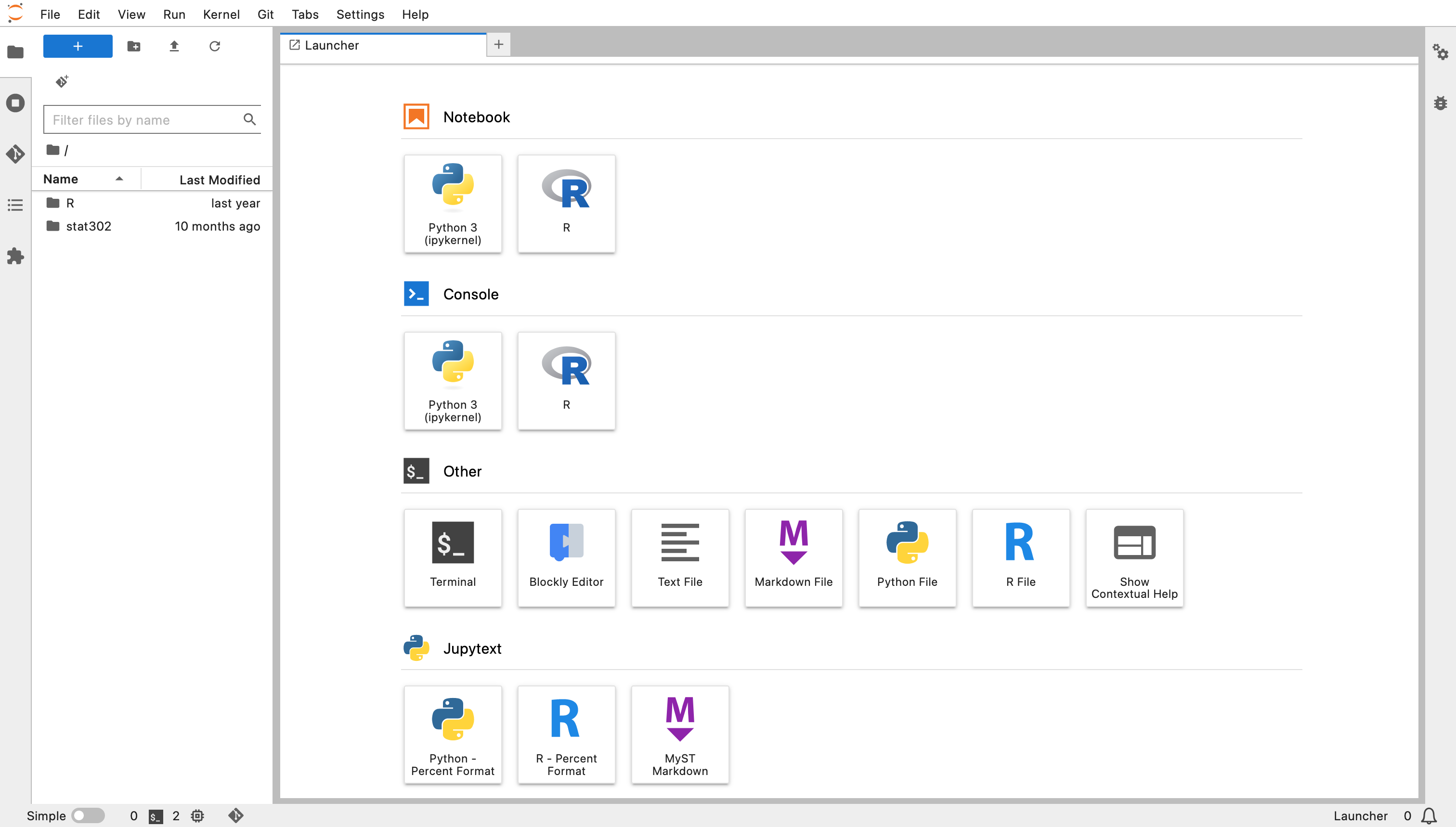
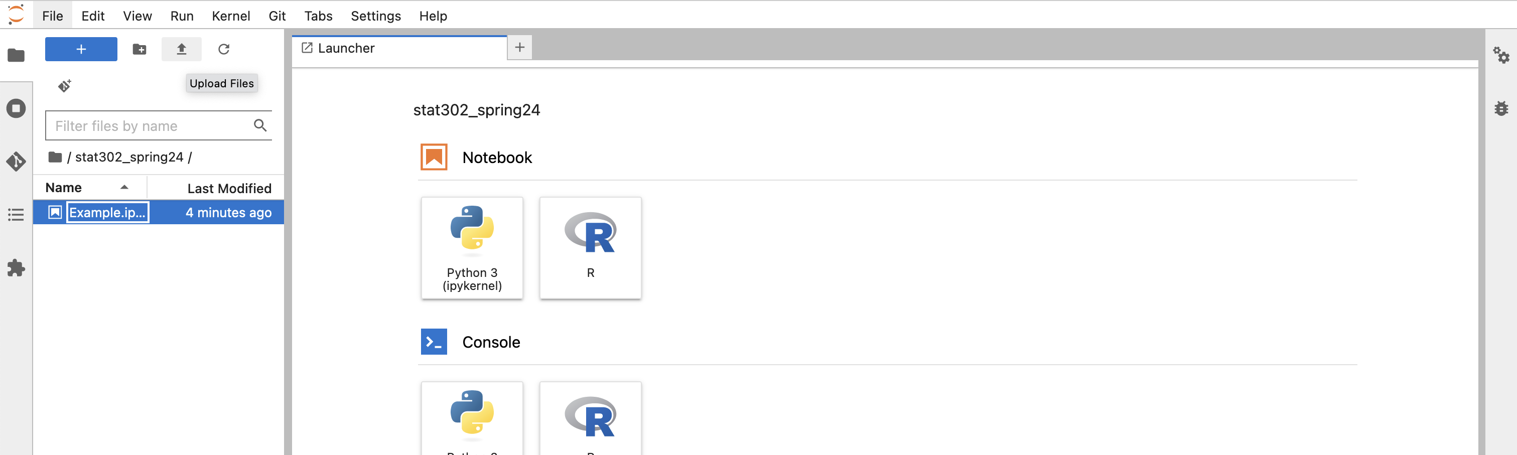
Create a new folder using the New Folder button on the left and call it Stat_302 and open that folder.
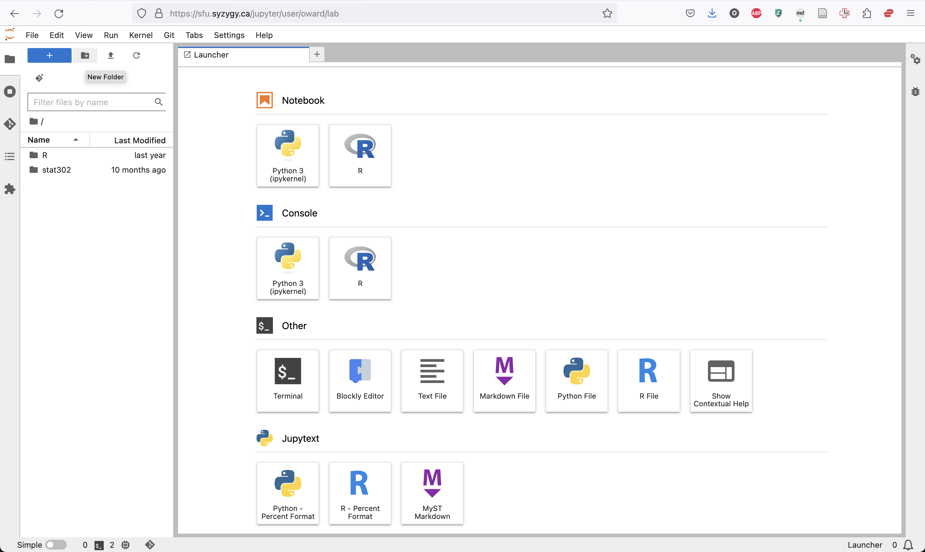
Inside that folder (by double clicking on the folder) create a new R notebook. This will create a new notebook in whichever folder you currently have open.
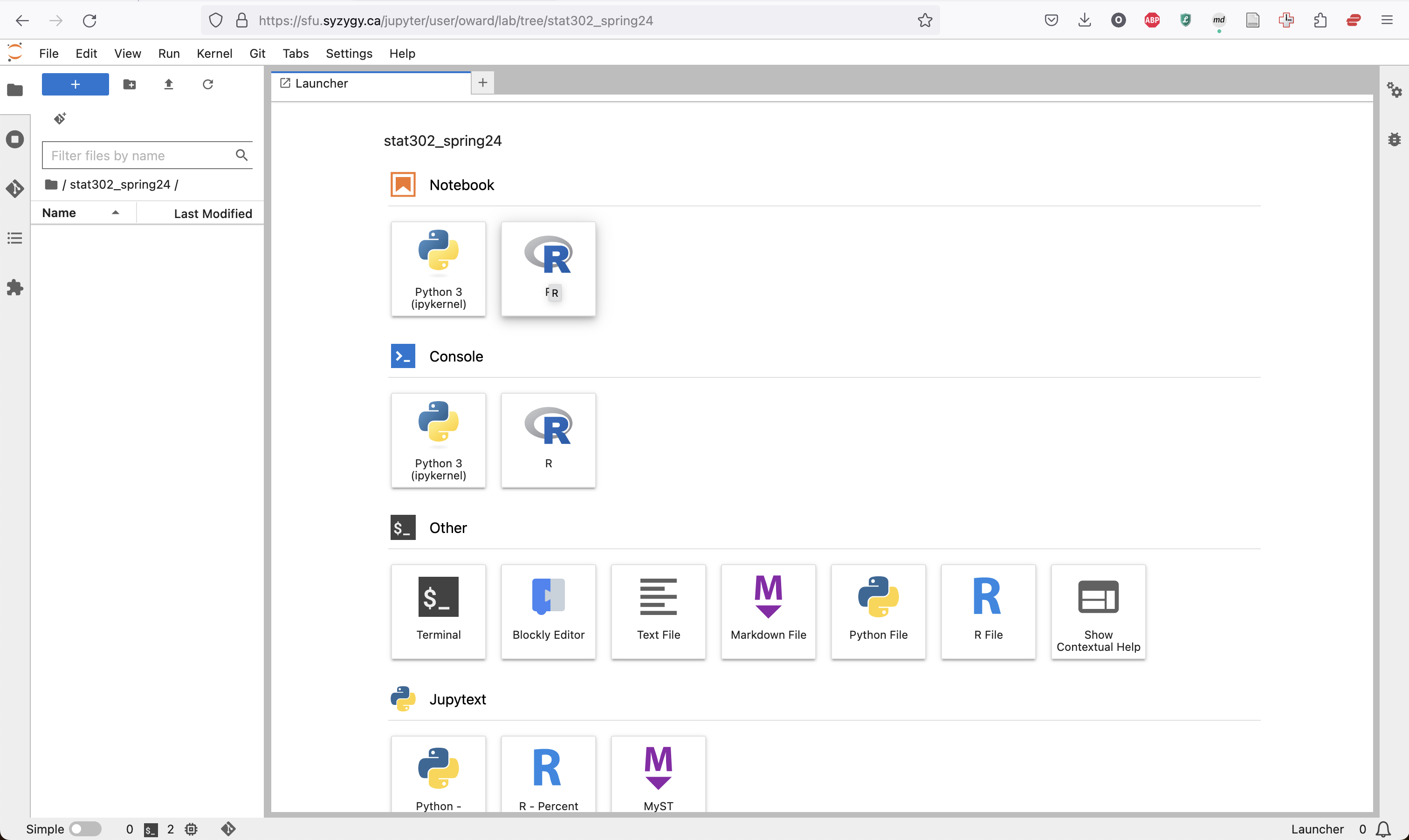
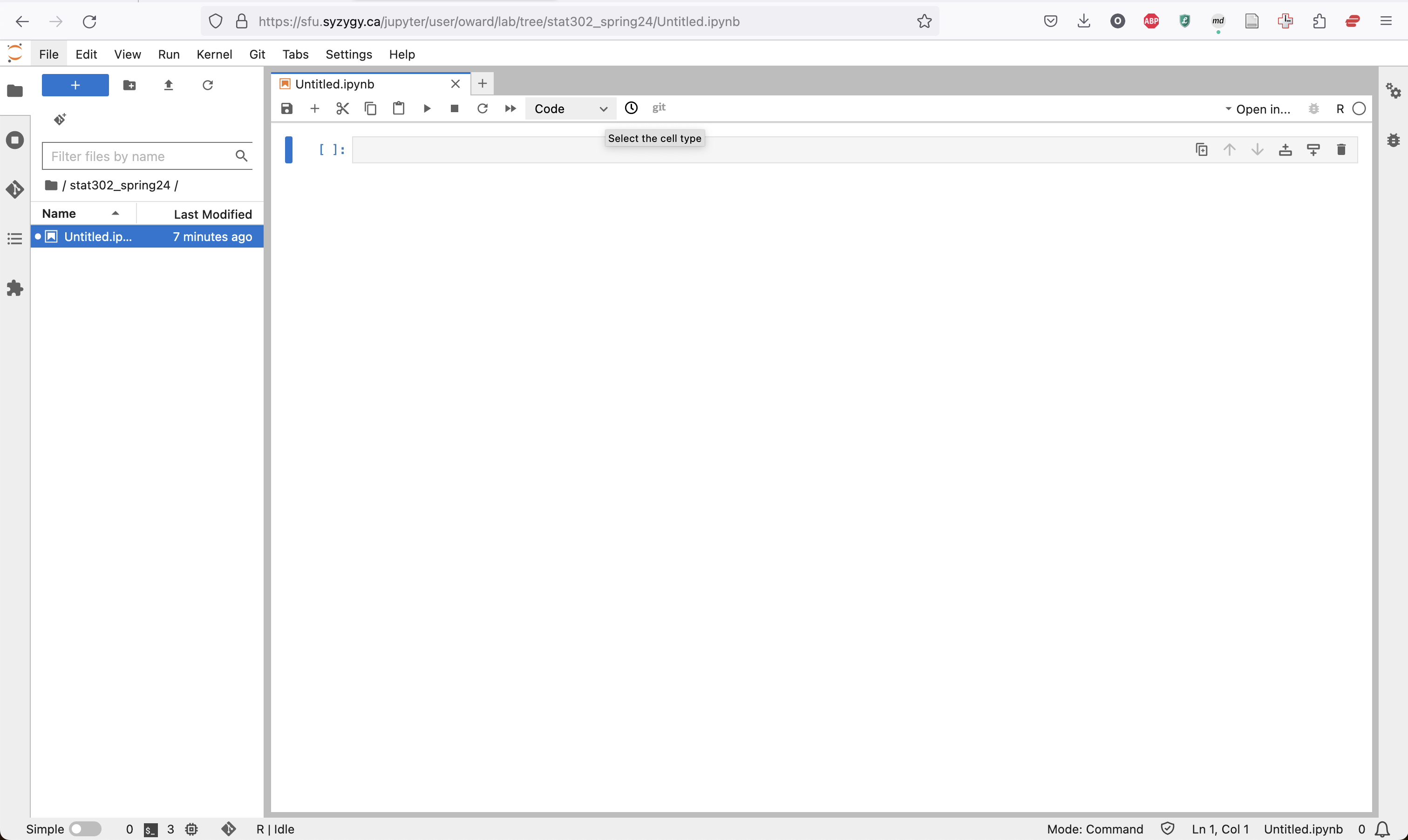
The new notebook will appear almost completely blank, with one initial cell.
![]()
Code can be entered in this line and run by pressing Command/Ctrl + Enter
or the Run button.

You can add a new line of code by pressing the Plus button.
When you do simple calculations the output will appear below the cell in Jupyter.
2 + 3[1] 54/5[1] 0.8sqrt(23)[1] 4.795832R has lots of built in functions to do mathematical and statistical tasks.
sqrt(4)[1] 2exp(10)[1] 22026.47You can find out more about a function by using ?. This will bring up a help page
?sqrtOften we want to store a value or a number so that we can reuse it. For example, if we think we will need sqrt(30) again later, we can store it as a variable. We do this using the <- operator. Note that the use of = is discouraged (for good reasons)!
sqrt_30 <- sqrt(30)

print(sqrt_30)
[1] 5.4772261 + sqrt_30[1] 6.477226sqrt_30/2[1] 2.738613This is a simple example but more important when you may have to do more complicated calculations. Names should be informative, to make it easier to remember what you might have called something!
What makes R most convenient is that it has lots of built in functions for doing statistics with common types of data. We will see the data formats which will appear in this class here. We have already seen how we can store a single data point as a variable using
one_gpa <- 3.7but we can do this with more complicated data also.
Suppose we instead want to store multiple data points, such as the gpa of 5 students in the class. We can actually store all of these in a single object called a vector. We create these using the c() function. We seperate values using ,.
gpas <- c(3.7, 2.9, 4.0, 3.1, 3.6)We can see all the values in this object by running
gpas[1] 3.7 2.9 4.0 3.1 3.6## or alternatively, same output
print(gpas)[1] 3.7 2.9 4.0 3.1 3.6We can see how many values we have stored using the length() function.
length(gpas)[1] 5What if we just want to use a single value from this object, say the second gpa?
We can extract specific elements using []. For example:
gpas[2] # returns just the second value[1] 2.9gpas[4] # just the 4th value[1] 3.1gpas[1:3] # the first 3[1] 3.7 2.9 4.0We can also perform operations on all the values. For example, to get the average gpa:
mean(gpas)[1] 3.46## we would get the same value doing this by hand
## remember the definition of the mean/average?
sum(gpas)/length(gpas)[1] 3.46Suppose instead of having a single gpa for each student, we had their gpa across 2 semesters. How could we store that?
gpa_1 <- c(3.7, 2.9, 4.0, 3.1, 3.6)
gpa_2 <- c(3.5, 3.3, 3.9, 3.4, 3.9)
So this means student 1 had a GPA of 3.7 in the first semester and a GPA of 3.5 in the second, and so on.
We would store this using a dataframe.
gpa_df <- data.frame(gpa_1, gpa_2)

gpa_df
gpa_1 gpa_2
1 3.7 3.5
2 2.9 3.3
3 4.0 3.9
4 3.1 3.4
5 3.6 3.9This data.frame is now a table of data, with 5 rows (the number of GPA’s we had for each semester) and 2 columns (the number of semesters).
Each row is a student (observation) and each column is a semester GPA (variable).
If we just want the information about the third student, we can again access that, in a similar way to before.
gpa_df[3, ] gpa_1 gpa_2
3 4 3.9Here because we have rows and columns we have two entries we can select. So if we want the entry in the second row and the first column we would use
gpa_df[2, 1][1] 2.9## or the 4th row, second column
gpa_df[4, 2][1] 3.4If we want all entries in a row, we leave the column choice blank, and vice versa for all entries in a column.
## gives us the entire first row
gpa_df[1, ]
gpa_1 gpa_2
1 3.7 3.5## gives us the entire 2nd column
gpa_df[, 2][1] 3.5 3.3 3.9 3.4 3.9We can extract a specific variable using the name of the data frame followed by $ and then the variable we are interested in.
Lets see what variables we have in gpa_df. As each variable is a column, we can check this using colnames.
colnames(gpa_df)[1] "gpa_1" "gpa_2"So to access all values in gpa_1, we can use
gpa_df$gpa_1[1] 3.7 2.9 4.0 3.1 3.6This way of accessing variables, using $ is useful when we have many variables in our data frame.
One slight annoyance with using Jupyter is that when you type gpa_df$, it does not prompt the possible options. Other platforms such as RStudio will give you the possible options.
We can also do things like compare the average GPA for each student and for each semester. R has lots of nice built in functions for tasks such as these.
## to get each students average GPA
rowMeans(gpa_df)
[1] 3.60 3.10 3.95 3.25 3.75## to get the average gpa for each semester
colMeans(gpa_df)gpa_1 gpa_2
3.46 3.60 To find out more about a specific R function you can place a ? in front of the name of the function. This will open a help page with examples of how to use it. Try running the following two examples to see this.
?mean
?expPerhaps the biggest advantage of using R for statistics is that there have been thousands of packages written to perform specific statistical tasks.
We can install packages using the install.packages command. You only need to run this the first time you install a package.
## only run this the first time, note the quotes around the package name
# install.packages("palmerpenguins")
After a package has been installed we can then load it using the library command.
library(palmerpenguins)Sometimes we will use a tibble instead of a dataframe. Tibbles are essentially just a more modern version and can be printed in a nicer format.
To do this we need to load the tidyverse suite of packages (assuming it has been installed previously).
library(tidyverse)── Attaching core tidyverse packages ──────────────────────── tidyverse 2.0.0 ──
✔ dplyr 1.1.3 ✔ readr 2.1.4
✔ forcats 1.0.0 ✔ stringr 1.5.0
✔ ggplot2 3.5.0 ✔ tibble 3.2.1
✔ lubridate 1.9.2 ✔ tidyr 1.3.0
✔ purrr 1.0.2
── Conflicts ────────────────────────────────────────── tidyverse_conflicts() ──
✖ dplyr::filter() masks stats::filter()
✖ dplyr::lag() masks stats::lag()
ℹ Use the conflicted package (<http://conflicted.r-lib.org/>) to force all conflicts to become errorsas_tibble(gpa_df)# A tibble: 5 × 2
gpa_1 gpa_2
<dbl> <dbl>
1 3.7 3.5
2 2.9 3.3
3 4 3.9
4 3.1 3.4
5 3.6 3.9Everything we have done so far has consisted of simple commands which are only one line long. An important skill is being able to save your code so that you can use it again. To do that, we can save code to several file types.
This section is how you will submit your homeworks for this class
We will first go through a simple example where you take an empty file and create the file you need to submit on Crowdmark. We will then repeat this for HW0.
If you are using Jupyter, the format of submitting is described here.
This is described in detail in the stats workshop canvas site, in the introduction file on the page R in Jupyter, however, the server may now look different to what is posted there.
As above, to use Jupyter you visit the website here and log in using your SFU credentials.
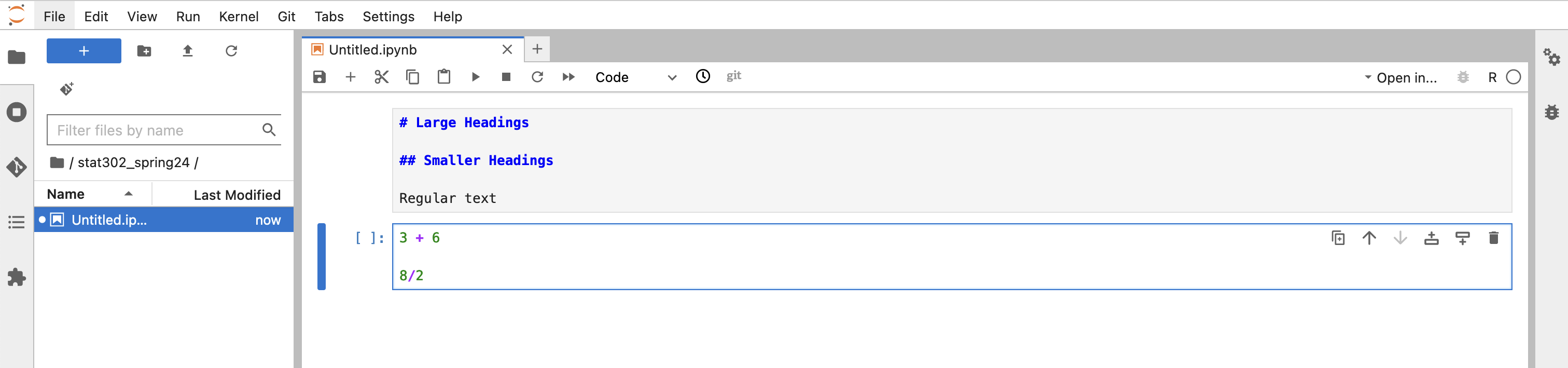
If you want to add some text (not a comment), between your code you can change the type of the box.
For example, if you want to format your file to have a heading and some text as well as code.

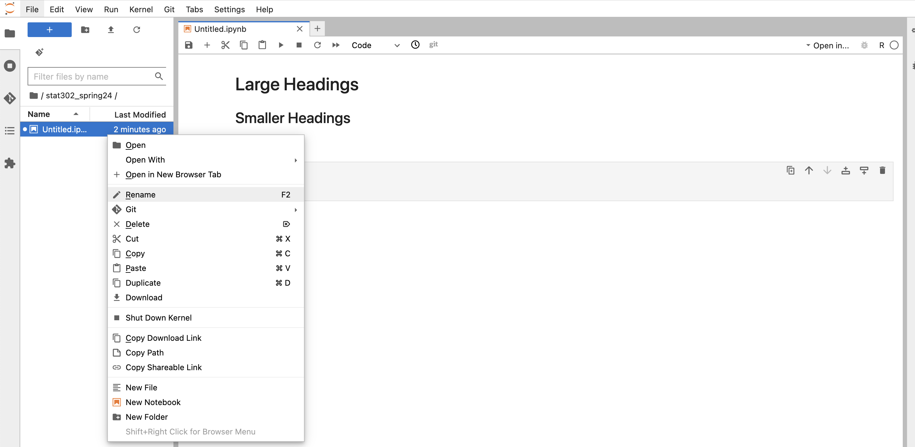
You should give this file a useful name, which can be done by right clicking on the name (Untitled) on the left side.
Finally, to save this file, such as for uploading it to crowdmark, click on File and then Save and Export Notebook as and select PDF. This will download a pdf file to your computer. You should save this to a folder where you can find it, so that you can then submit it to crowdmark.
For homeworks, I will give you an outline file which you will need to upload to Jupyter, edit, and then download as a pdf before uploading to Crowdmark.
This will be explained below.
To submit your homework with Jupyter there will be 4 steps you must repeat.
First you must download the homework file from Canvas. This will be in the files section, in the Homeworks folder.
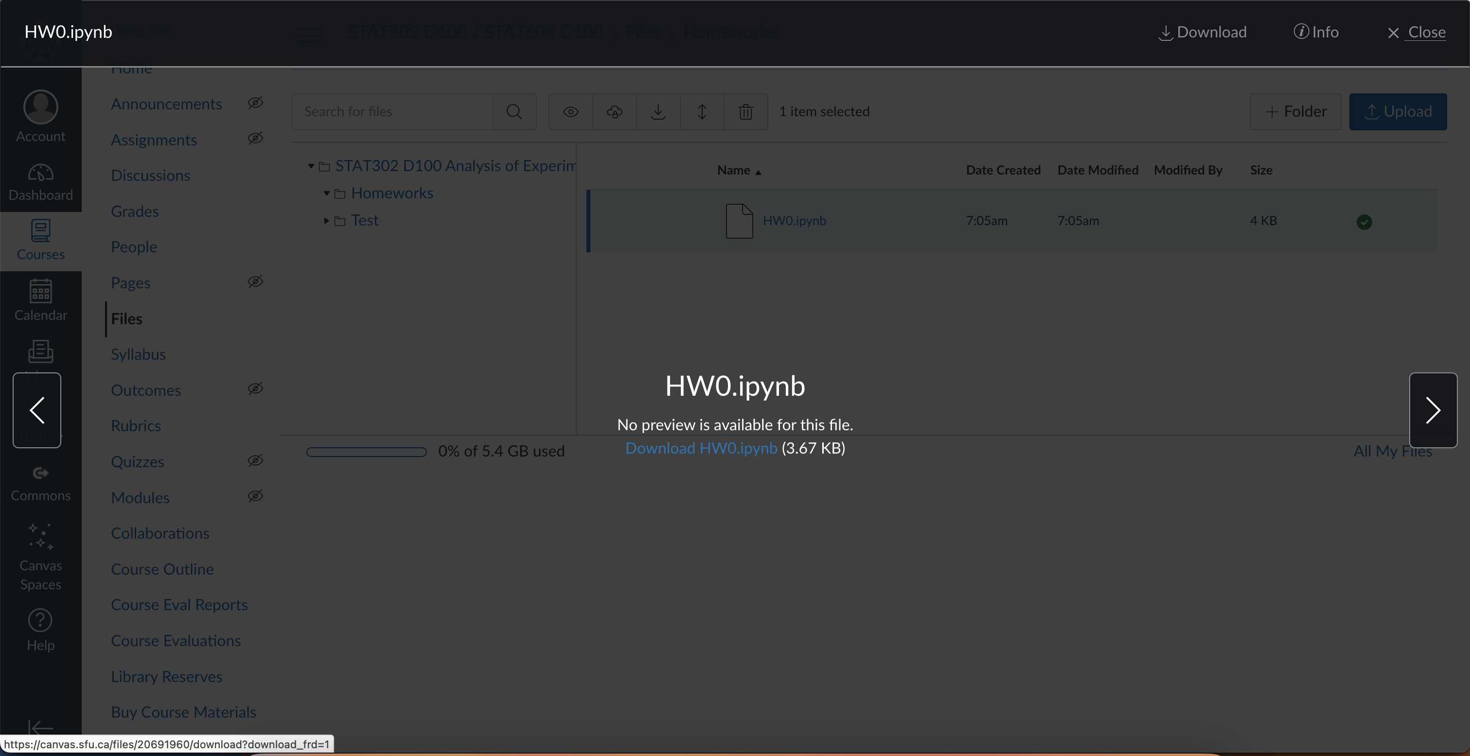
Save the file somewhere on your computer where you can easily find it, because you will then upload it to Jupyter.
To do this, after signing into Jupyter and entering the folder you created for this class, click the upload button in the top left.
Select the file you just downloaded from Canvas and click upload. You can then open this file in jupyter. You should rename it to be of the form FirstName_LastName_HWNumber.ipynb.
After you have completed working on the notebook, you should download it as a pdf (see above). You then upload that pdf to Crowdmark.
Please check the pdf looks as you expect before uploading it.
You will also have the option to complete and submit your homeworks using RStudio, by knitting an Rmd file. However, this has some slight issues which you need to be aware of, and you must ensure you deal with them in preparing your submission.
Note that when using RStudio, code chunks (similar to cells in Jupyter) are available only for code, and text will be written directly into the Rmd file. Be sure not to miss text questions in the homework, which will not be inside cells.
If you Knit an Rmd file, this will create a HTML document. This is almost in the format we want to submit, except we need to convert it to pdf. To do this, when it is open in the browser you should Print it to PDF, saving it with the correct name.
This pdf should then be submitted to crowdmark. Note that from HW1 on, you will be asked to submit separate pages for each question. Using Jupyter will automatically split questions across pages, however this is not possible in RStudio (without additional installation). As such, you must ensure that you submit the correct pages of the pdf for each of the questions.
Comments
We can write comments by beginning a line of code with the character
#.