
4 ANOVA
4.1 Introduction
We have already seen a little bit of ANOVA in terms of linear regression, but we will first go back even a step further and see the connection between a two sample t-test and ANOVA. In its simplest form, ANOVA can be used to check if the means of groups differ.
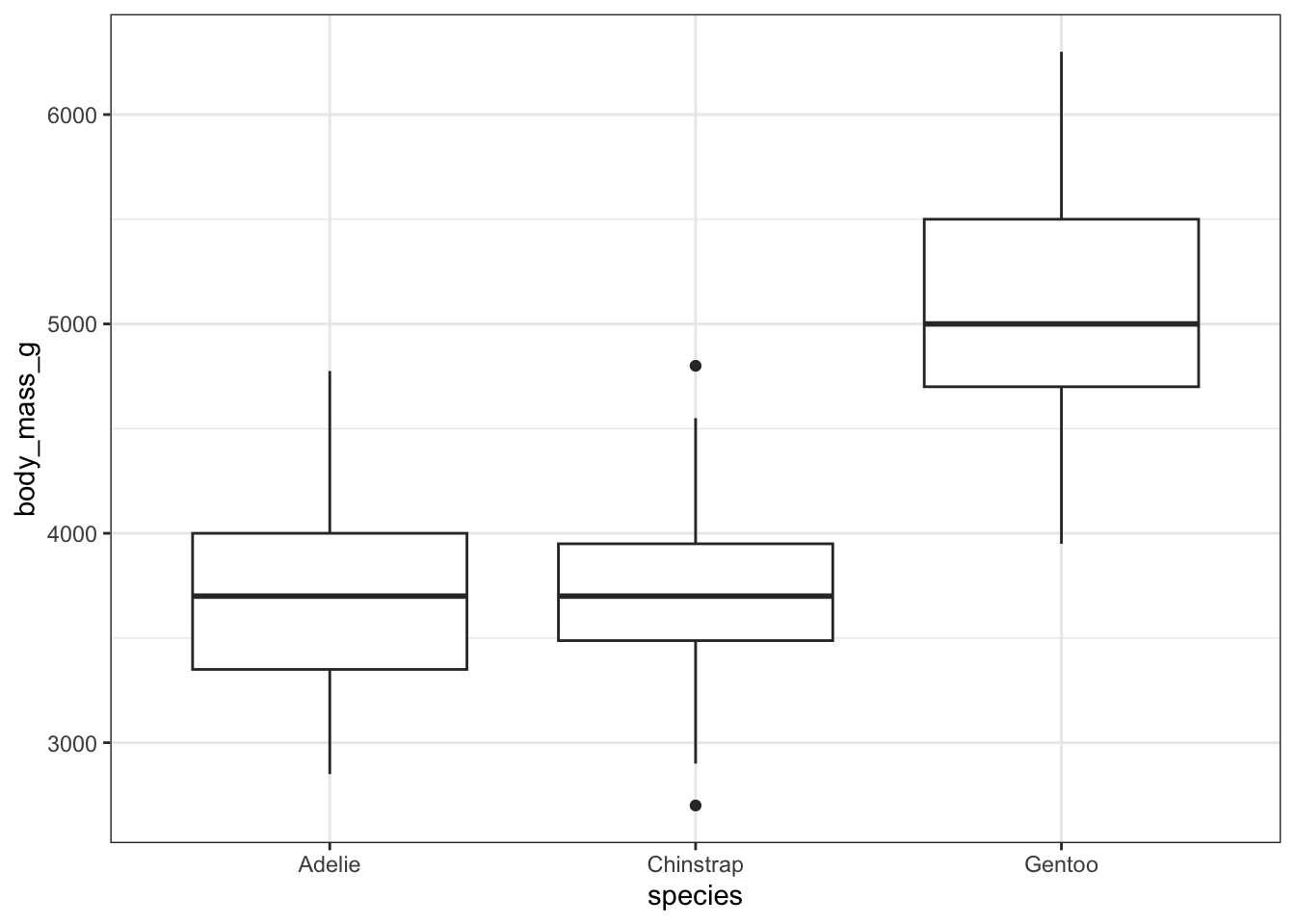
One of the advantages of using ANOVA compared to doing a t-test is that ANOVA allows us to compare multiple groups all at once. If we tried to do this using multiple t-tests, we would quickly run into a problem of multiple testing, which we will finally discuss below. When we fit linear regression models our outcome \(Y\) was numeric while we had both numeric and categorical predictors. If we only had a single categorical predictor, then this would result in a regression where we get a different horizontal line for each of the categories. This is more commonly done using a box-plot for each of the categories. ANOVA is a way of testing if the mean of the \(Y\) variable in all these categories is the same. It can also be used to do more complicated tests, some of which we will see later.
Previously we saw that we could check if the mean weight of Adelie penguins and Gentoo penguins was the same by doing a 2 sample t-test. If we assume the variance is the same in both groups, with sample means \(\bar{x}_1\) and \(\bar{x}_2\) and sample variances \(s_1^2\) and \(s_2^2\) from \(n_1\) and \(n_2\) samples, our test statistic is
\[ t =\frac{\bar{x}_1-\bar{x}_2}{s_p \sqrt{\frac{1}{n_1}+ \frac{1}{n_2}}}, \]
where
\[ s_p = \sqrt{\frac{(n_1-1)s_1^2 + (n_2 - 1)s_2^2}{n_1 + n_2 - 2}}. \]
Under \(H_0\), \(t\) follows a t-distribution with \(n_1+n_2-1\) degrees of freedom. However, this would only tell us if Adelie and Gentoo penguins are different. If we do another t-test, to compare Gentoo and Chinstrap or Adelie and Chinstrap penguins, then we run into multiple testing. We will see later why multiple testing is such a problem, but for now you just need to know that it messes everything up. Thankfully, we can instead use ANOVA.
In this chapter we will see an introduction to ANOVA including one-way and two-way ANOVA, along with how we can use ANOVA with regression for more specific hypothesis tests than those we saw before.
4.2 One Way ANOVA
In one-way ANOVA we are interested in testing if the mean of some quantitative response is the same across a categorical variable. We will observe data in \(J\) different groups. In each of these groups \(j=1,2,\ldots,J\) we observe \(n_1,n_2,\ldots, n_J\) data points. We will say that \(n_T = \sum_{j=1}^{J}n_j\), is the total number of observations, in all groups. For example, in the penguin example we have \(J=3\) and the following observations in each group.
table(penguins$species)
   Adelie Chinstrap    Gentoo
      152        68       124
We will say our observed data is \(Y_{ij}\) where \(j\) tells us which group the observation is in and \(i\) says it is the \(i\)-th observation in that group. For example \(Y_{12}\) is the first observation in the second group (category) and \(Y_{21}\) is the second observation in the first group (category).
The One-Way ANOVA Model says that we can write a model for each \(Y_{ij}\) as
\[ Y_{ij} = \mu + \alpha_j + \epsilon_{ij}, \]
where we have:
\(\mu\) is an overall mean, which is common to all observations,
\(\alpha_j\) is a group level effect within group \(j\),
\(\epsilon_{ij}\) is an individual observation level error, similar to the errors we saw in regression models, which we discuss more shortly. We will call this version of the model the effects model. We will see a small modification to this when we fit this model in
Rbelow.
Note that we can also write this as
\[ Y_{ij} = \mu_j + \epsilon_{ij}, \]
where we have \(\mu_j = \mu + \alpha_j\). This is just an equivalent way of writing the same model. We will call this the means model. We want to test the hypothesis that the mean in each of these groups is the same. Using the means model, this is equivalent to saying we want to test
\[ H_0:\mu_1=\mu_2=\ldots=\mu_J \ vs\ H_A: \text{one}\ \mu_j\ \text{differs from rest}. \]
Writing this in terms of the effects model, this is equivalent to saying
\[ H_0:\alpha_1=\alpha_2=\ldots=\alpha_J=0 \ vs\ H_A: \text{one}\ \alpha_j\neq 0. \]
These are just two slightly different ways of writing the same model. If this is a reasonable model for the data, then we can use ANOVA to perform these hypothesis tests. This will be very similar to checking the regression conditions. However, before we do that, lets see in a bit more detail how we write out the test statistic for this model.
If this model is familiar and reminds you of fitting a linear regression then that is correct. We can think of this as just fitting an intercept, so a horizontal line only, for each group and seeing if we need a different intercept for each of the groups.

To do this, we compute the squared sums of errors and get a test statistic. We compare the residual sum of squares and the model sum of squares, which we can get using the total sum of squares.
The residual sum of squares will be a measure of how much the data varies around the individual group means (the blue lines). If each group has a different mean \(\mu_j\) we will estimate this quantity with the sample mean for that group
\[ \hat{\mu}_j = \frac{1}{n_j}\sum_{i=1}^{n_j}Y_{ij} = \bar{y}_j, \]
the mean of the samples in the \(j\)-th group. Then, the residual for each observation will be the difference between the value and the group mean,
\[ e_{ij} = y_{ij} - \bar{y}_j, \]
for each observation \(i\) in group \(j\). The residual sum of squares will be the sum of the square of all residuals, over all data in each of the groups,
\[ SSError = \sum_{j=1}^{J}\sum_{i=1}^{n_j}(y_{ij} - \bar{y}_j)^2. \]
Similarly, the total sum of squares is a measure of the variability around the overall mean (the red line). We write \(\bar{y}\) to be the mean of all observations,
\[ \bar{y} = \frac{1}{J}\sum_{j=1}^{J}\bar{y}_j, \]
i.e, the mean of the group means is the overall mean. Then the total sum of squares is
\[ SSTotal = \sum_{j=1}^{J}\sum_{i=1}^{n_j}(y_{ij} - \bar{y})^2. \]
Finally, we also have the model sum of squares. This quantifies the variability of the fitted values around the overall mean, and is given by
\[ SSModel = \sum_{j=1}^{J}\sum_{i=1}^{n_j}(\hat{y}_{ij} - \bar{y})^2. \]
Now note that our model is that \(Y_{ij} = \mu_j +\epsilon_{ij}\) so our estimate for \(\hat{y}_{ij}\) is \(\bar{y}_j\). Now, if we think about a single group, we will have for every \(i\) that
\[ \hat{y}_{ij} = \bar{y}_j, \]
i.e we will have the same estimate for each observation in a given group. So for each group we will be summing up the same thing \(n_j\) times,
\[ SSModel = \sum_{j=1}^{K}\sum_{i=1}^{n_j}(\bar{y}_j - \bar{y})^2 = \sum_{j=1}^{J}n_j(\bar{y}_j - \bar{y})^2. \]
As we saw previously we can again write that
\[ SSTotal = SSModel + SSError. \]
We need to examine how many degrees of freedom these quantities have. In \(SSTotal\), we are only estimating the overall mean, so we have \(n_T - 1\) degrees of freedom. For \(SSError\), we have to estimate the \(J\) group means, so that has \(n_T - J\) degrees of freedom. This means that we must have \(J-1\) degrees of freedom for \(SSModel\), as they have to match like the equation for the sums of squares.
We then need to compute the mean squared errors, which is the sum of squares errors divided by their degrees of freedom. This gives us
\[ MSModel = \frac{SSModel}{J -1}, \]
and
\[ MSError =\frac{SSError}{n_T - J}. \]
Finally, our test statistic is then
\[ f = \frac{MSModel}{MSError}. \]
Recall our null and alternative hypothesis for this problem. If our null hypothesis is true then \(f\) should follow an \(F\) distribution with \(J-1, n_T-J\) degrees of freedom. If our value of \(f\) is unlikely to be from such a distribution then we would reject the null and conclude that not all the group means are the same.
Now we want to see how to do this hypothesis test in R. As already mentioned, this is somewhat like a linear regression with no slope and just a different intercept for each category. This is actually how we will fit this model in R. To use ANOVA, we first create the corresponding regression fit.
spec_fit <- lm(body_mass_g ~ species, data = penguins)

summary(spec_fit)
Call:
lm(formula = body_mass_g ~ species, data = penguins)

Residuals:
     Min       1Q   Median       3Q      Max
-1126.02  -333.09   -33.09   316.91  1223.98

Coefficients:
                 Estimate Std. Error t value Pr(>|t|)
(Intercept)       3700.66      37.62   98.37   <2e-16 ***
speciesChinstrap    32.43      67.51    0.48    0.631
speciesGentoo     1375.35      56.15   24.50   <2e-16 ***
---
Signif. codes:  0 '***' 0.001 '**' 0.01 '*' 0.05 '.' 0.1 ' ' 1

Residual standard error: 462.3 on 339 degrees of freedom
  (2 observations deleted due to missingness)
Multiple R-squared:  0.6697,    Adjusted R-squared:  0.6677
F-statistic: 343.6 on 2 and 339 DF,  p-value: < 2.2e-16
Now we need to be a bit careful about how to interpret this output, and figure out how exactly relates to the model we considered above. Recall that we said we can write this model as
\[ Y_{ij} = \mu + \alpha_j + \epsilon_{ij}. \]
If we fix \(\alpha_1 = 0\) then we are actually estimating the \(J\) possible parameters, because that means that \(\mu_1 = \mu\) and \(\mu_2 = \mu + \alpha_2, \mu_3 = \mu + \alpha_3\), etc. This is just like a linear regression with a different intercept for each of the possible categories! So \(\alpha_2\) tells us how group 2 differs from group 1, and so on. So in this regression model the Intercept is \(\hat{\mu}\), speciesChinstrap is \(\hat{\alpha}_2\), and speciesGentoo is \(\hat{\alpha}_3\). These quantities are all we need to do the \(F\) test and indeed summary gives us the result we need. However, we will soon need the anova function, so we will see how we can use that here, and how to understand its output.
The ANOVA Table
Using anova with a correctly specified linear regression gives us the ANOVA table, which contains all the information we need for all possible ANOVA problems.
anova_fit <- anova(spec_fit)
anova_fit
Analysis of Variance Table
Response: body_mass_g
Df Sum Sq Mean Sq F value Pr(>F)
species 2 146864214 73432107 343.63 < 2.2e-16 ***
Residuals 339 72443483 213698
---
Signif. codes: 0 '***' 0.001 '**' 0.01 '*' 0.05 '.' 0.1 ' ' 1The first line of this output shows the model sums of squares and mean squares, which is the sum of squares divided by the degrees of freedom. The second line shows the same quantities for the error sum of squares. The ratio of the mean sums of squares gives the F test statistic and the corresponding \(p\)-value.
Just like in regression, ANOVA is fitting a model to our data and we need to check the conditions of that model. Remember that we said
\[ Y_{ij} = \mu_j + \epsilon_{ij}. \]
We have conditions on these errors which need to be satisfied for an ANOVA model to be reasonable and to allow us to actually trust the results. These are quite similar to what we saw in linear regression.
When we fit an ANOVA model, we get residuals
\[ e_{ij} = y_{ij} - \hat{y}_{ij} = y_{ij} - \bar{y}_j. \]
We should investigate 4 conditions of these residuals:
That the residuals have mean 0. This is always the case
That the variance of the residuals in each group is the same
That the residuals are normally distributed with some common variance
That the residuals are independent
We can only check some of these directly. The residuals will always have mean zero, as we saw with regression. We can only really check the independence condition if we know how the raw data was collected. However the other two conditions can be checked, in much the same way as we did this in regression.
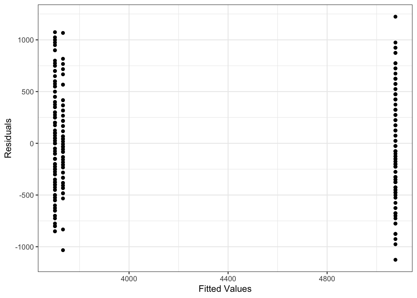
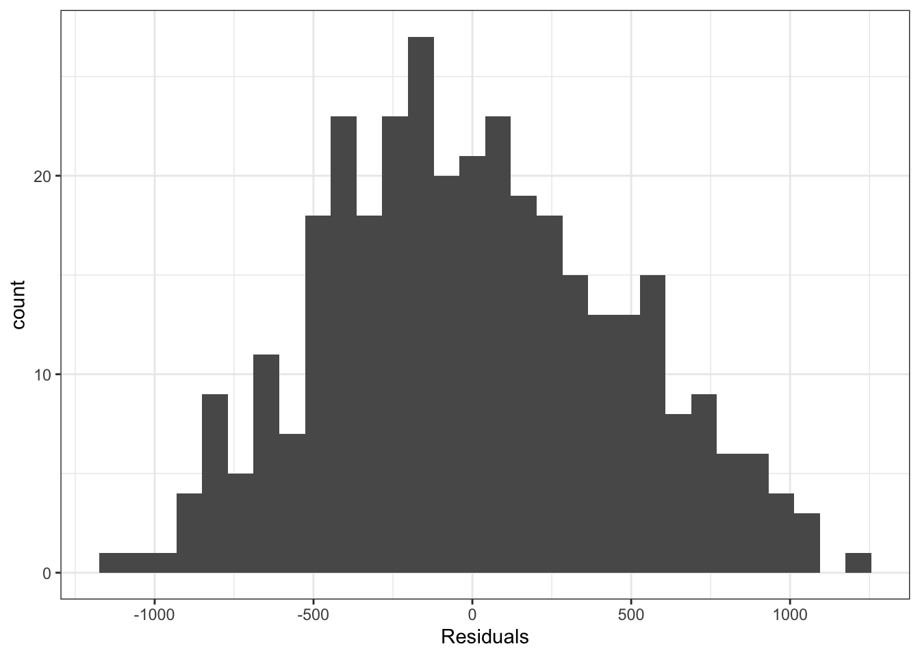
To check the variance of the residuals, we can plot them against the fitted values, just as we did in regression. Now, because we just have a different mean for each group, the data in each group will lie on a vertical line. The spread of the points in these lines will tell us how the variance looks. Note that plotting a histogram of the residuals may also be useful.
Similarly, we can use the same normal quantile plot to investigate whether the normality assumption is reasonable.
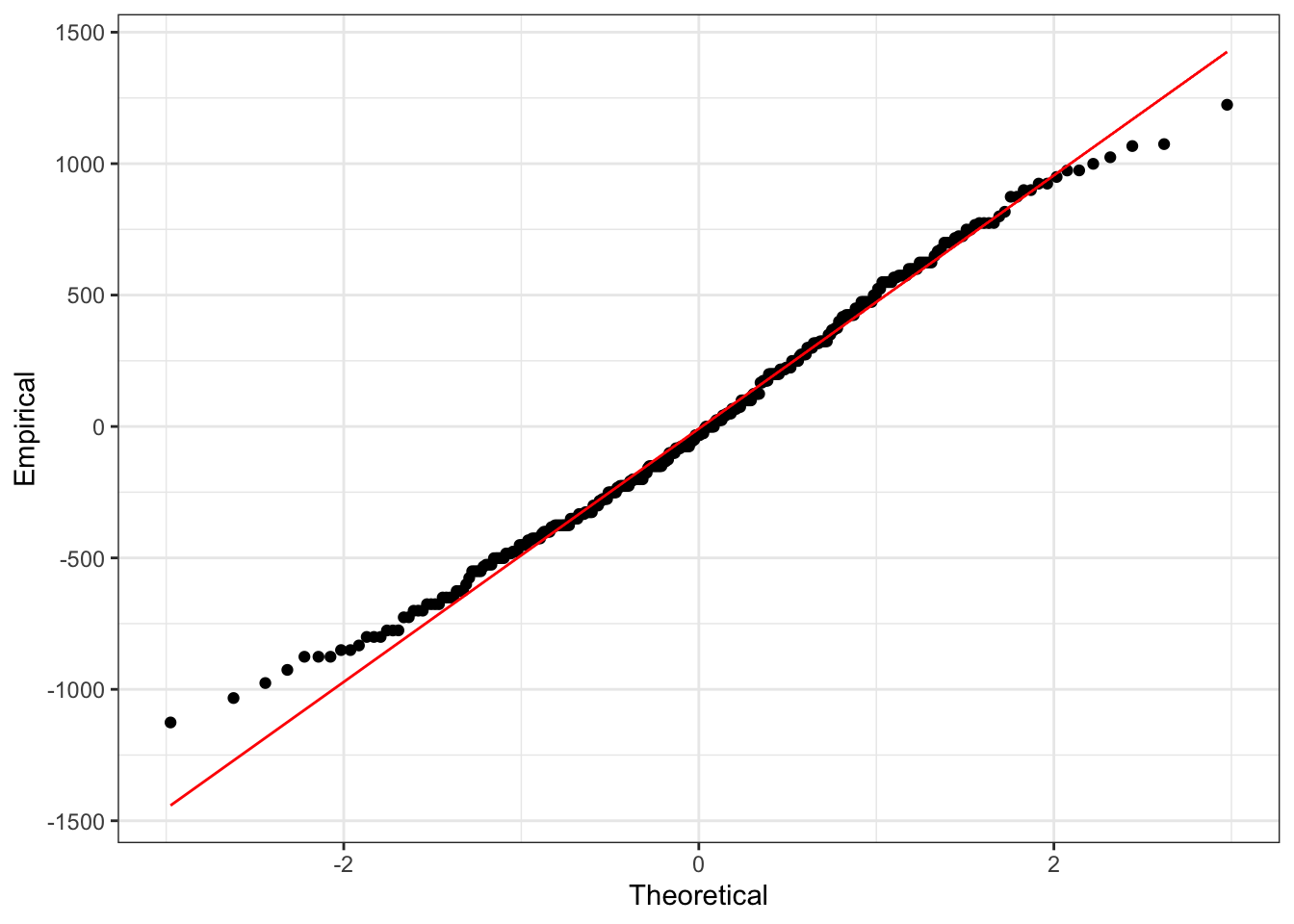
Looking at these plots we don’t see any clear reasons to think the assumptions of an ANOVA model are violated here. This means we can interpret the results, and conclude that not all group means are equal.
Creating these plots in R, is identical to how we did this before and we can just the regression model we used in ANOVA.
plot(spec_fit$fitted.values, spec_fit$residuals)
qqnorm(spec_fit$residuals)
qqline(spec_fit$residuals, col = "red")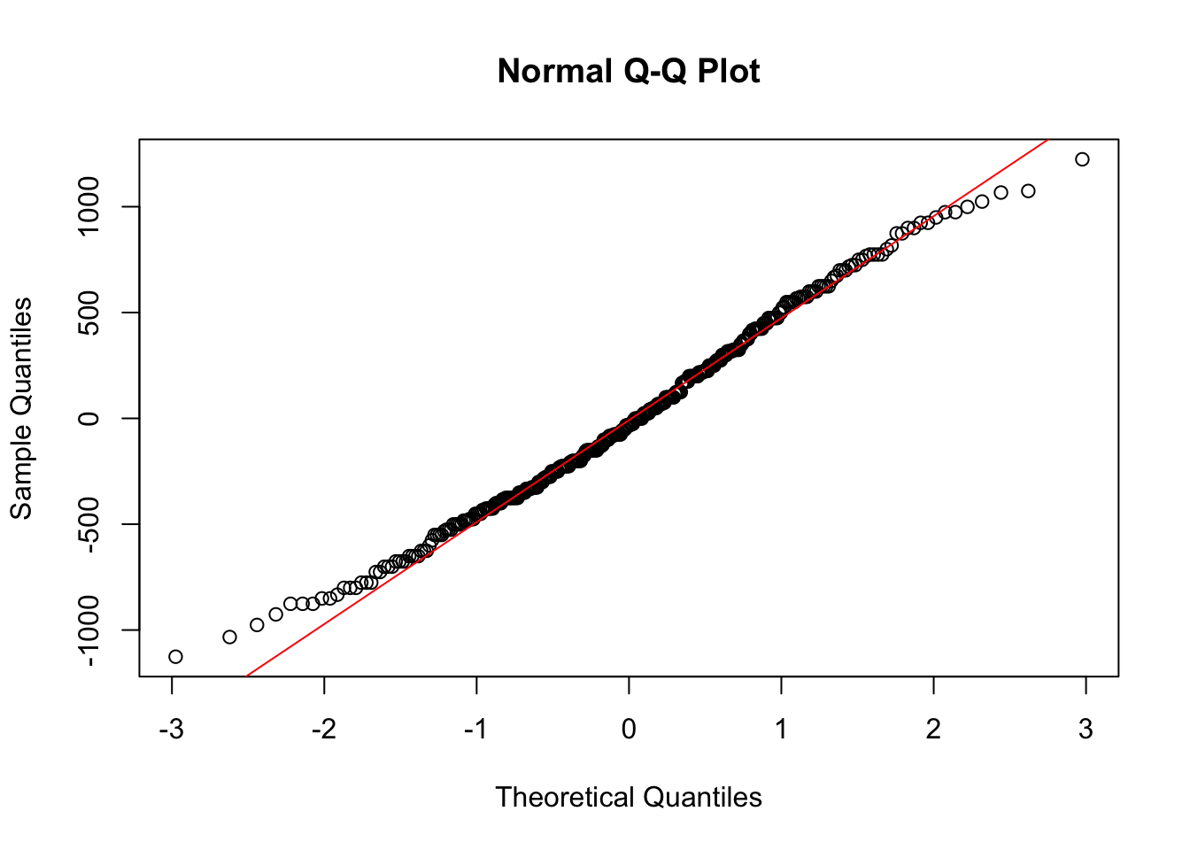
Note that if you can compute the sample standard deviation of the residuals within each group, one informal check that the variability is the same across groups is to look at the ratio of the largest sample standard deviation to the smallest. If this is less than 2, then this is evidence that a common variance assumption across groups is reasonable.
Example
Lets see another example where we need to check these assumptions. Remember that we should check these after fitting the regression and before doing the ANOVA. For this example we want to examine whether one-way ANOVA is appropriate to understand the differences in tail lengths across three of the most common species of Hawks in North America (Red Tailed, Coopers, Sharp Shinned). We can fit the regression model corresponding to ANOVA and then look at the residuals.
library(Stat2Data)
data(Hawks)


hawk_fit <- lm(Tail ~ Species, data = Hawks)

summary(hawk_fit)
Call:
lm(formula = Tail ~ Species, data = Hawks)

Residuals:
     Min       1Q   Median       3Q      Max
-100.149  -10.149   -0.149    9.851   74.276

Coefficients:
            Estimate Std. Error t value Pr(>|t|)
(Intercept)  200.914      1.809  111.08   <2e-16 ***
SpeciesRT     21.235      1.915   11.09   <2e-16 ***
SpeciesSS    -54.190      2.037  -26.61   <2e-16 ***
---
Signif. codes:  0 '***' 0.001 '**' 0.01 '*' 0.05 '.' 0.1 ' ' 1

Residual standard error: 15.13 on 905 degrees of freedom
Multiple R-squared:  0.8315,    Adjusted R-squared:  0.8311
F-statistic:  2233 on 2 and 905 DF,  p-value: < 2.2e-16

Looking at these plots, we see that the assumptions required to use ANOVA are not reasonable for this data. There are some possible outliers in the histogram, the variance seems to vary quite a bit from group to group and the quantile plot has some points far from the line. So we need an alternative model here, which we will see later.
Remember what this \(F\)-test tells us, and, as importantly, what it doesn’t tell us! If we reject \(H_0\) then we conclude that there is evidence to reject that all groups have the same mean. But that’s all it says. It could be the case that two of the 3 groups have the same mean, but the \(F\)-test would still give us this result.
If we wanted to conclude which groups are different, you might think we could do a bunch of different two sample t-tests. However, this is back to the problem (again!) of multiple testing. Now we will finally see some more detail on this, and one thing we can do to avoid it for this problem.
The problem of multiple testing
Recall that when we do a hypothesis test, we can still make a mistake. We could conclude the null should be rejected when the null is actually correct (Type 1 Error) or we could fail to reject the null when it should have been rejected (Type 2 Error). The significance level \(\alpha\), controls the type 1 error. So if we do a single hypothesis test at \(\alpha=0.05\), that means, the probability of a Type 1 error is \(0.05\). If we could collect a random sample of data from a population 100 times, each time doing a hypothesis test on one variable, we would expect to reject \(H_0\) 5 times, even if it is true.
n_rep <- 100
p <- 0.95

test_results <- sample(0:1, size = n_rep, replace = TRUE, prob = c(p, 1-p))

sum(test_results)
[1] 5Suppose now instead we do 2 hypothesis tests on this data, for two different variables. Again, the truth is that all these null hypothesis tests are true. Now, how many times do we reject the null?
n_tests <- 2
n_rep <- 1000

## the first hyp
test_results_1 <- sample(0:1, size = n_rep, replace = TRUE, prob = c(p, 1-p))
## the second hyp
test_results_2 <- sample(0:1, size = n_rep, replace = TRUE, prob = c(p, 1-p))

all_tests <- test_results_1 + test_results_2

## the proportion of times we reject H0
sum(all_tests  > 0)/n_rep
[1] 0.109Now, we reject the null approximately 10% of the time, more than 100 times if we could repeat this 1000 times. This will become even more of a problem if we do more tests. For example, we could do 10 hypothesis tests (don’t worry if the code is confusing, its just to illustrate the point).
n_tests <- 10
n_rep <- 1000

results <- matrix(NA, nrow = n_tests, ncol = n_rep)

for(i in 1:n_tests){
  results[i,] <- sample(0:1, size = n_rep, replace = TRUE, prob = c(p, 1-p))
}

all_tests <- apply(results, 2, sum)

sum(all_tests  > 0)/n_rep
[1] 0.396No we will reject at least one null hypothesis approximately 40% of the time, even though all the null hypotheses are correct!
The probability we make at least 1 Type 1 error is known as the family wise error rate. When we do more than 1 hypothesis test this will increase, and can get large quickly! This is one of the contributors to what is known as the reproducibility crisis, where people repeat scientific experiments and are not able to replicate famous results.
Problems like this have led different scientists to conclude, using the exact same raw data, that certain drugs are both increasing and not increasing your risk of adverse health, i.e, they could get completely different results! If you are a scientist, you should be aware of these issues!
If we want to do multiple hypothesis tests then we need to be able to control the family wise error rate. One way to do this is to decrease the type 1 error. If the type 1 error for each test is \(\alpha=0.005\) then the family wise error will be \(1-(0.995)^{10}\approx 0.05\). There are many important ways to do this. Here, we will just see one way to account for this within ANOVA.
Tukey’s HSD Test
When we do ANOVA for an example such as this, we would like to then be able to say something about the pairwise differences in the groups. Tukey’s Honest significant difference (HSD) test is one way to do this, which preserves the family wise confidence level of at least 95%. If we want to decrease the family wise error we need to decrease \(\alpha\) for each test. Similarly, if we want 95% family wise confidence then we need to make each individual confidence interval wider.
The formula for these confidence intervals between groups \(k\) and \(l\) will be
\[ \bar{y}_k -\bar{y}_l \pm q \hat{\sigma}_e\sqrt{\frac{1}{n_k}+\frac{1}{n_l}}. \]
These intervals will ensure the family wise confidence is at least \(100(1-\alpha)\%\). We have not explained how to compute \(q\) here, because in practice we can use a function in R to construct these intervals. To do this we need to first use the aov function on the regression fit, and then the TukeyHSD function on this output.
TukeyHSD(aov(spec_fit), conf.level = 0.95) Tukey multiple comparisons of means
95% family-wise confidence level
Fit: aov(formula = spec_fit)
$species
diff lwr upr p adj
Chinstrap-Adelie 32.42598 -126.5002 191.3522 0.8806666
Gentoo-Adelie 1375.35401 1243.1786 1507.5294 0.0000000
Gentoo-Chinstrap 1342.92802 1178.4810 1507.3750 0.0000000This gives us each of the pairwise confidence intervals for the difference between two groups. We also get a \(p\)-value for whether the difference between these two groups is zero or not. We can also show these differences and the confidence intervals visually using plot.
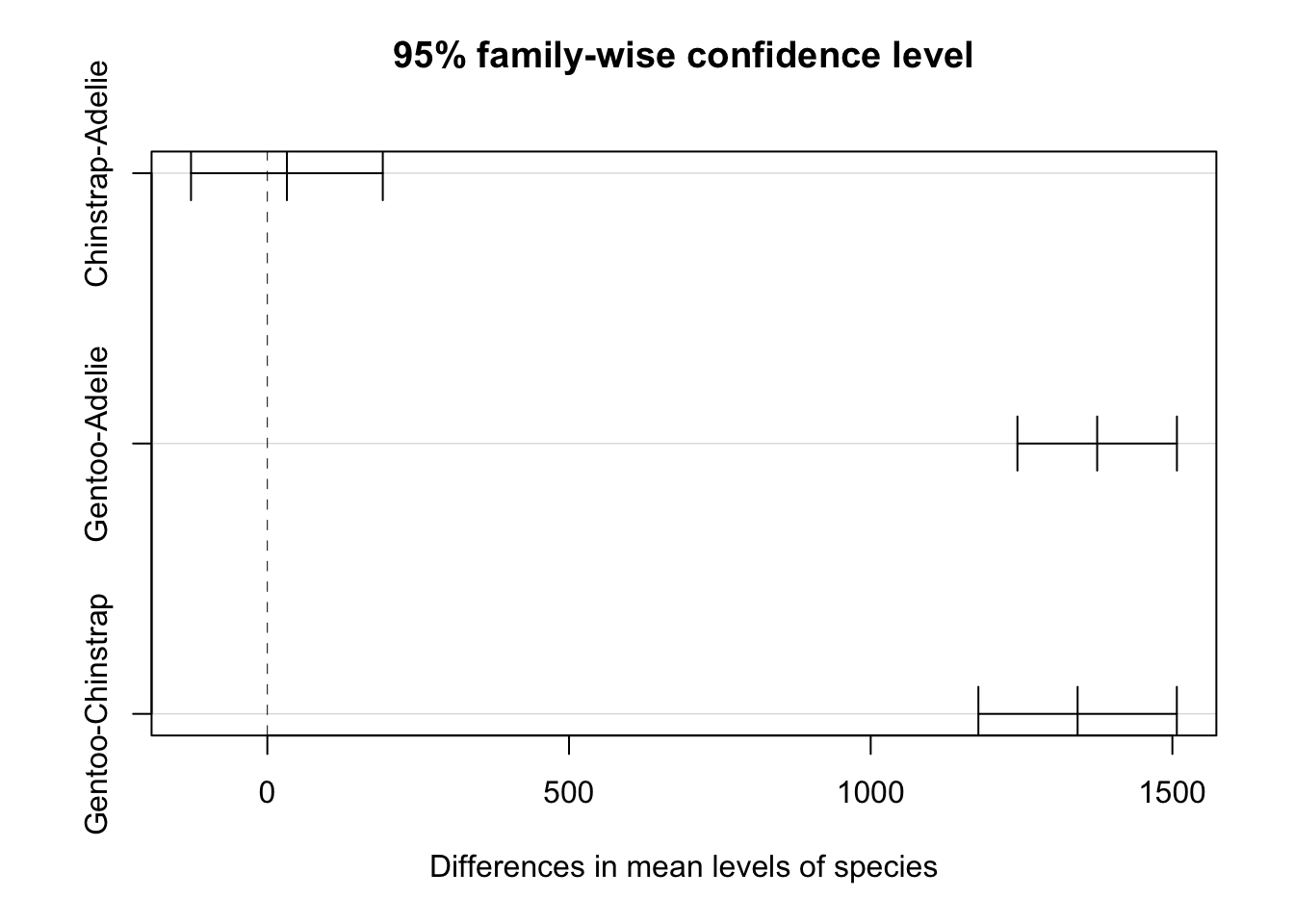
We see here that this indicates that the difference between Chinstrap and Adelie penguins may in fact be 0, however the difference between Gentoo and the other species is clearly different from 0.
When using an F-test and Tukey’s test, we might not reject \(H_0\) using an F-test, but if we then used Tukey’s test we might still identify differences between pairs. This is because Tukey’s test is not equivalent to the \(F\)-test, whereas if we have only two groups the two sample \(t\)-test is exactly the same as the \(F\)-test. In general, the standard way to use these two tests is to first use the \(F\)-test, then only use the Tukey test to examine pairwise differences if the null is rejected by the \(F\)-test.
Lets finish this section with some more examples of using ANOVA and checking the conditions for ANOVA.
Example
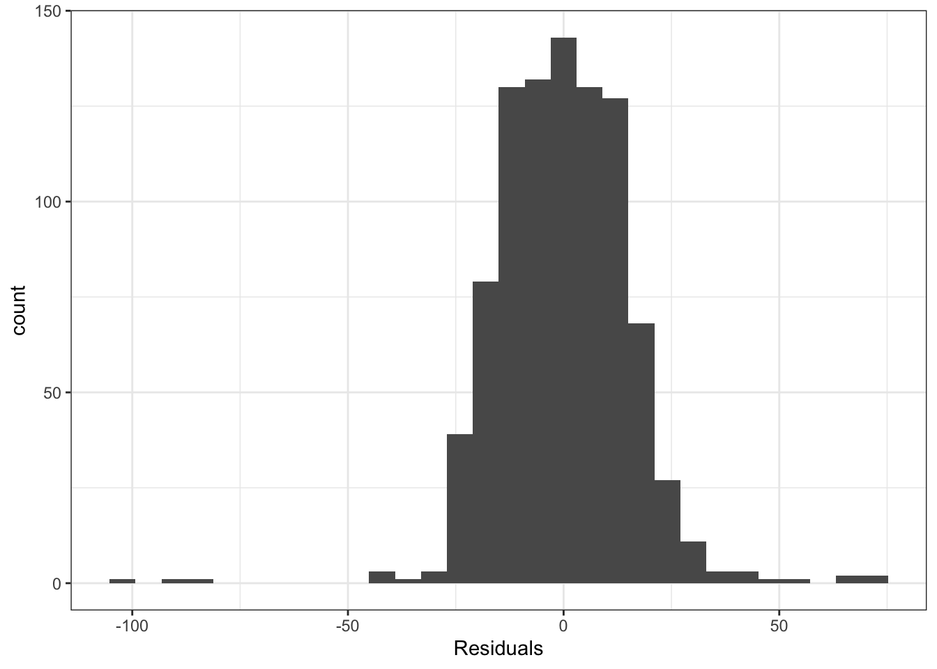
For the Hawk data above we compared tail lengths. We could also compare the length of the Culmen, a part of the beak of a bird. To compare the group means for this variable across the three species we again run our regression against the categorical variables only, and examine the resulting residuals.
reg_fit <- lm(Culmen ~ Species, data = Hawks)

plot(reg_fit$fitted.values, reg_fit$residuals)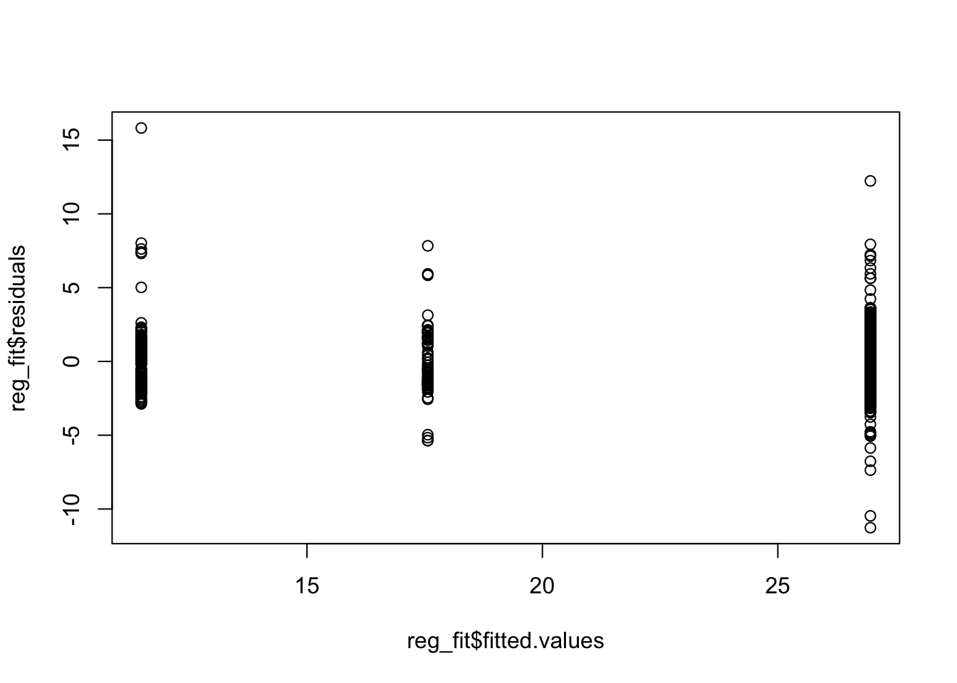
qqnorm(reg_fit$residuals)
qqline(reg_fit$residuals, col = "red")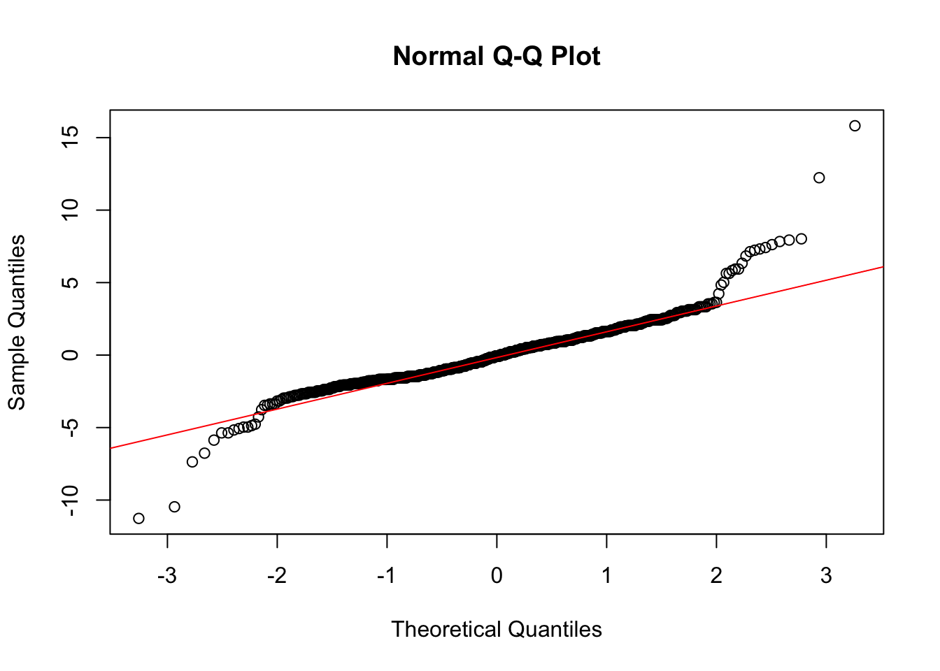
We see clear problems in these residuals plots, indicating the variance is not constant and the normal assumption for the errors is not reasonable. So we cannot proceed with using ANOVA.
Example
For another example, we consider the survival time of Cancer patients with 1 of 5 different organs affected by cancer. We would like to see if the average survival time differs across the organ affected. As before, we can try fit a standard one-way ANOVA model by first fitting the model in lm in checking the residuals.
data("CancerSurvival")

cancer_fit <- lm(Survival ~ Organ, data = CancerSurvival)

plot(cancer_fit$fitted.values, cancer_fit$residuals)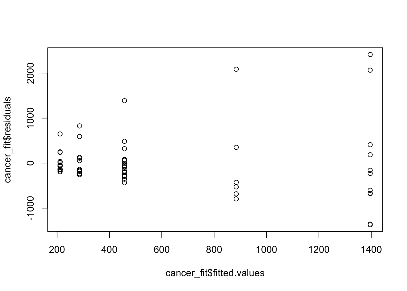
qqnorm(cancer_fit$residuals)
qqline(cancer_fit$residuals, col = "red")
These residuals indicate some problems with the model. One thing to keep in mind here is that survival time will always be non negative. Much like income it may make sense to take a (natural) log transformation of it, and refit the model.
log_fit <- lm(log(Survival) ~ Organ, data = CancerSurvival)

plot(log_fit$fitted.values, log_fit$residuals)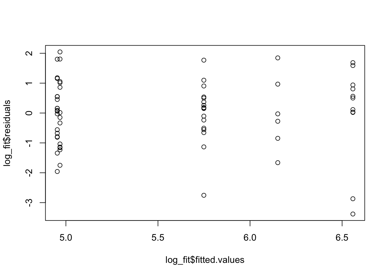
qqnorm(log_fit$residuals)
qqline(log_fit$residuals, col = "red")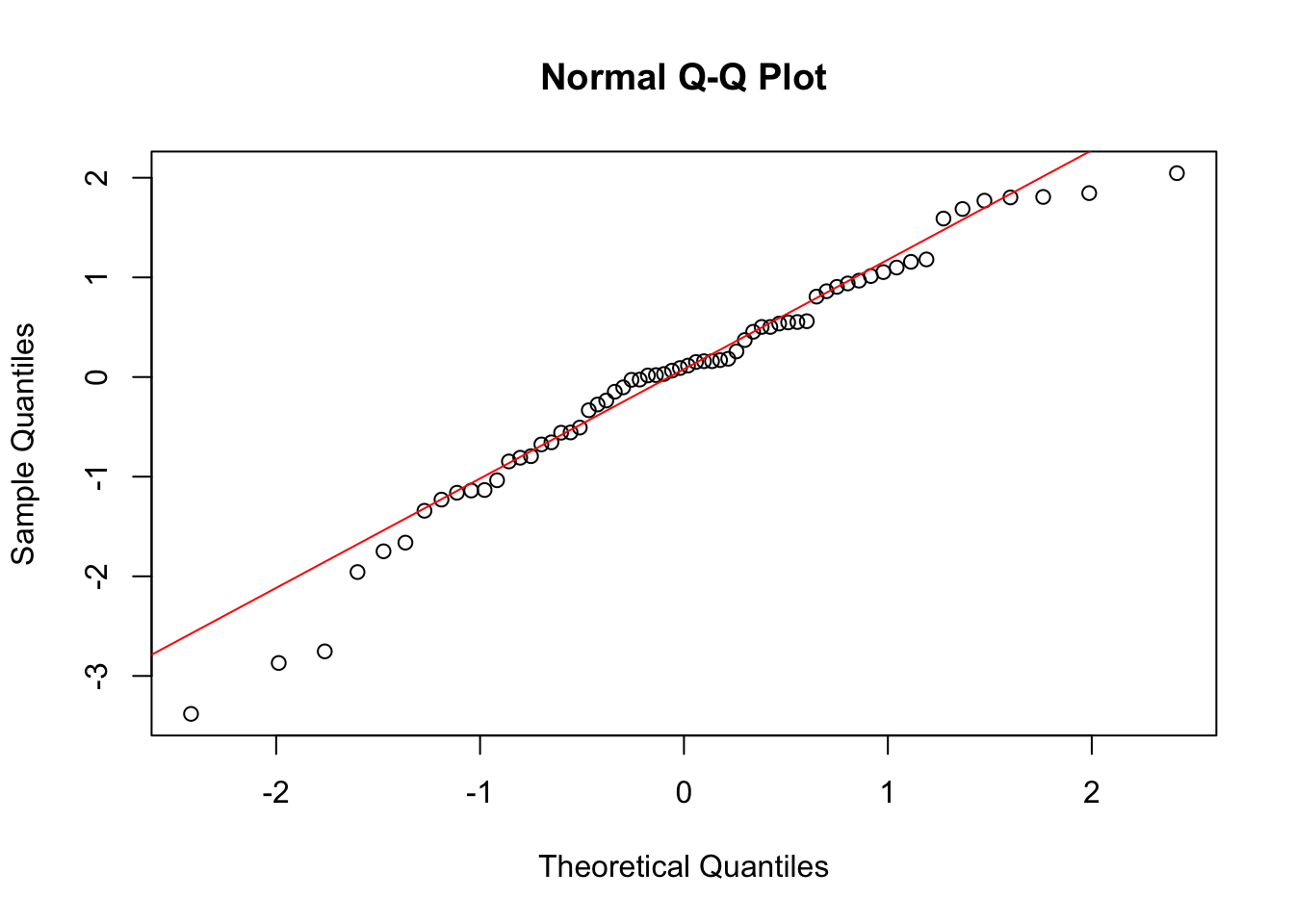
While these residuals are still not perfect, we do see that the regression assumptions look more reasonable when we consider the log of the survival time as our response variable. Let’s do ANOVA and interpret the results.
Now our ANOVA model is that
\[ \log(Y_{ij}) = \mu_j + \epsilon_{ij}, \]
and we want to test if all the \(\mu_j\) are equal or not, at \(\alpha=0.01\), for example.
anova(log_fit)Analysis of Variance Table
Response: log(Survival)
Df Sum Sq Mean Sq F value Pr(>F)
Organ 4 24.487 6.1216 4.286 0.004122 **
Residuals 59 84.270 1.4283
---
Signif. codes: 0 '***' 0.001 '**' 0.01 '*' 0.05 '.' 0.1 ' ' 1When we do this we get an F-test with a p-value of \(0.004 <\alpha\) so we reject our null and conclude the means in these groups are not all the same. We can then use Tukey’s test to investigate these differences further.
TukeyHSD(aov(log_fit), conf.level = 0.95) Tukey multiple comparisons of means
95% family-wise confidence level
Fit: aov(formula = log_fit)
$Organ
diff lwr upr p adj
Bronchus-Breast -1.60543320 -2.906741 -0.3041254 0.0083352
Colon-Breast -0.80948110 -2.110789 0.4918267 0.4119156
Ovary-Breast -0.40798703 -2.114754 1.2987803 0.9615409
Stomach-Breast -1.59068365 -2.968399 -0.2129685 0.0158132
Colon-Bronchus 0.79595210 -0.357534 1.9494382 0.3072938
Ovary-Bronchus 1.19744617 -0.399483 2.7943753 0.2296079
Stomach-Bronchus 0.01474955 -1.224293 1.2537924 0.9999997
Ovary-Colon 0.40149407 -1.195435 1.9984232 0.9540004
Stomach-Colon -0.78120255 -2.020245 0.4578403 0.3981146
Stomach-Ovary -1.18269662 -2.842480 0.4770864 0.2763506Now when we get these confidence intervals for the pairwise differences, of which there are 10 possibilities, we see that most of these intervals contain 0, indicating no difference between those two groups. Only one interval, the first, has a small \(p\)-value and evidence for a difference.
4.3 Two Way ANOVA
We have seen how we can use one-way ANOVA to examine how a numeric variable varies across a single categorical variable. We’ve also seen that this model doesn’t always work either. One of the reasons that the assumptions are not reasonable for a one-way ANOVA model are that there could be an interaction with another categorical variable, which we have not accounted for. Accounting for this will give us a model which can correctly describe how \(Y\) varies. This is how we incorporate a second factor variable into ANOVA, giving a two-way ANOVA model.
Adding categorical predictors
We now want to consider a model where we have 2 categorical predictors. The notation gets a little bit more complicated to do this.
We will have two categorical variables, where the first variable has \(I\) possible categories and the second has \(J\) possible categories. For example in the penguin data we could have the first categorical variable being species, giving \(I=3\), and the second being sex, giving \(J=2\)
So \((i,j)\) is a combination of the two categorical variables. We will have \(n_{ij}\) observations with first variable (or factor) equal to \(i\) and second equal to \(j\).
We say that \(Y_{ijk}\) is the \(k\)-th observation with category \(i\) in the first variable and category \(j\) in the second variable. For the penguin data this means \(Y_{ijk}\) is the \(k\)-th penguin in the \(i\)-th species and the \(j\)-th sex.
Now, the general two-way ANOVA model we will consider here is given by
\[ Y_{ijk} = \mu +\alpha_i +\beta_j +\gamma_{ij} + \epsilon_{ijk}. \]
We now have an overall mean \(\mu\) along with an effect for each of the two categorical predictors, and the interaction between those two predictors. The errors \(\epsilon_{ijk}\) are all independent and we want them to all be from the same normal distribution with some fixed variance.
We call \(\alpha\) the main effects of the first categorical variable (or factor) and \(\beta\) the main effects of the second factor. Then \(\gamma\) is the interaction effects between those two predictors.
Again we could also write this as a means version, which would be given by
\[ Y_{ijk} = \mu_{ij} + \epsilon_{ijk}. \]
To allow interpretation (and fitting) of these models we will again enforce that some of these coefficients are zero. In particular we will have
- \(\alpha_1 =0\)
- \(\beta_1 = 0\)
- \(\gamma_{1j}=0\) for all values of \(j\)
- \(\gamma_{i1}=0\) for all values of \(i\)
We will soon see how these assumptions are convenient for fitting the model and interpreting it.
Now, if we can estimate these parameters, we can interpret how changing these categorical predictors effects the outcome variable (\(Y\)). Lets consider interpreting these for the penguin example. For this, then we have \(I=3\), the three species (in alphabetical order) and \(J=2\) the two sexes (in alphabetical order). If \(i=1\) then we are talking about Adelie penguins. If \(j=1\) then we are talking about female penguins. Using the constraints then if \(i=j=1\) we have \(\alpha_1 = \beta_1 = \gamma_{11} = 0\) then the model is
\[ Y_{11k} = \mu +\epsilon_{ijk} \]
If we assume all the \(\gamma=0\) then we have no interaction effects. We will do this initially to make it easier to explain the output. Then if we have \(i=2\) and \(j=1\) the model is
\[ Y_{21k} = \mu + \alpha_2 + \epsilon_{21k}, \]
so \(\alpha_2\) gives information about the change in mean body mass from Adelie to Chinstrap penguins. So \(\alpha\) tells us about the effect of species on how the means vary.
Similarly, if we have \(i=1\) and \(j=2\) then
\[ Y_{12k} = \mu +\beta_2 +\epsilon_{12k}, \]
and \(\beta_2\) tells us how the mean body mass changes from female to male penguins. So \(\beta\) tells us about the effect of sex on how the group means vary.
We also need to interpret the interaction effects \(\gamma_{ij}\). If \(\gamma_{ij}=0\) for all \(i,j\) then there is no interaction between the two predictors. That means the effect of sex doesn’t change as we change species and similarly, that the effect of species doesn’t change as we change the sex variable.
If any \(\gamma_{ij}\neq 0\) that means that the effect of these categorical variables changes as we change categories of them. For example, the effect of sex can be different in different species. If there are interactions then it is a little harder to interpret these models. But it is, unsurprisingly, quite similar to when we added interactions to a linear regression.
Fitting two-way ANOVA
To make this model (slightly) easier to understand we will initially assume that there are no interaction effects, and so the ANOVA model is given by
\[ Y_{ijk} = \mu +\alpha_i +\beta_j + \epsilon_{ijk}. \]
Now, if we estimate the parameters of our model, we will get
\[ \hat{y}_{ij} = \hat{\mu} + \hat{\alpha}_i + \hat{\beta}_j, \] for each observation with the first categorical variable equal to \(i\) and the second equal to \(j\). Then, as before, we will have the error sum of squares given by
\[ SSError = \sum_{i=1}^{I}\sum_{j=1}^{J}\sum_{k=1}^{n_{ij}}(y_{ijk} - \hat{y}_{ij})^2, \]
and similarly the total sum of squares will be given by
\[ SSTotal = \sum_{i=1}^{I}\sum_{j=1}^{J}\sum_{k=1}^{n_{ij}}(y_{ijk}- \bar{y})^2, \]
where \(\bar{y}\) is the mean of all observations across all groups. Note that for \(SSError\) we will have \(n_T - IJ\) degrees of freedom. As before we can then write the model sum of squares as
\[ SSModel = SSTotal - SSError. \]
It turns out that if the data is balanced, meaning we have a similar number of observations in each of the possible categories, then we can write
\[ SSModel = SSA + SSB, \]
where \(SSA\) tells us how much of the variability in the response is explained by the first factor (the first categorical variable) and \(SSB\) is how much is explained by the second factor (the second categorical) variable.
We can see how many penguins are in each of the possible categories, to check if the balance assumption is ok.
# A tibble: 6 × 3
# Groups:   species [3]
  species   sex        n
  <fct>     <fct>  <int>
1 Adelie    female    73
2 Adelie    male      73
3 Chinstrap female    34
4 Chinstrap male      34
5 Gentoo    female    58
6 Gentoo    male      61
While we have slightly less Chinstrap penguins, there are still enough observations in each group that the data is somewhat balanced.
To compute these sums of squares for each factor, we again use a regression model, which will allow us to estimate \(\alpha\) and \(\beta\), and we can then check the conditions before getting the ANOVA table.
two_fit <- lm(body_mass_g ~ species + sex, data = na.omit(penguins))

summary(two_fit)
Call:
lm(formula = body_mass_g ~ species + sex, data = na.omit(penguins))

Residuals:
    Min      1Q  Median      3Q     Max
-816.87 -217.80  -16.87  227.61  882.20

Coefficients:
                 Estimate Std. Error t value Pr(>|t|)
(Intercept)       3372.39      31.43 107.308   <2e-16 ***
speciesChinstrap    26.92      46.48   0.579    0.563
speciesGentoo     1377.86      39.10  35.236   <2e-16 ***
sexmale            667.56      34.70  19.236   <2e-16 ***
---
Signif. codes:  0 '***' 0.001 '**' 0.01 '*' 0.05 '.' 0.1 ' ' 1

Residual standard error: 316.6 on 329 degrees of freedom
Multiple R-squared:  0.8468,    Adjusted R-squared:  0.8454
F-statistic: 606.1 on 3 and 329 DF,  p-value: < 2.2e-16
Now with \(\alpha_1 =\beta_1=0\) we have \(\hat{\mu}\) given by the intercept, \(\hat{\alpha}_2\) and \(\hat{\alpha}_3\) given by specieschinstrap and speciesGentoo and \(\hat{\beta}_2\) given by sexmale.
Before constructing the ANOVA table we check these residuals.
hist(two_fit$residuals)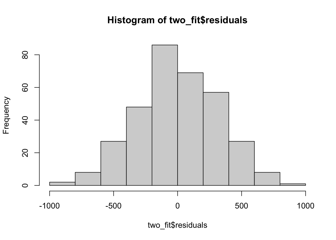
plot(x = two_fit$fitted.values, y = two_fit$residuals)
qqnorm(two_fit$residuals)
qqline(two_fit$residuals, col = "red")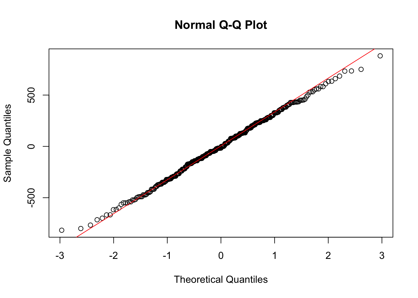
These residuals look mostly reasonable, so we can then construct the ANOVA table.
anova(two_fit)Analysis of Variance Table
Response: body_mass_g
Df Sum Sq Mean Sq F value Pr(>F)
species 2 145190219 72595110 724.21 < 2.2e-16 ***
sex 1 37090262 37090262 370.01 < 2.2e-16 ***
Residuals 329 32979185 100241
---
Signif. codes: 0 '***' 0.001 '**' 0.01 '*' 0.05 '.' 0.1 ' ' 1Now note that this table looks a bit different to what we had before. We now have 3 rows, one for each of the factors and one for the residuals. Similarly we now have 2 test statistics and 2 p-values. The sum of squares for species is \(SSA\) and the sum of squares for sex is \(SSB\).
Now the two test statistics are calculated using
\[ f_1 = \frac{MSA}{MSError} \mbox{ and } f_2 = \frac{MSB}{MSError}, \]
where the degrees of freedom for each is given in the corresponding row. For example,
\[ MSA = 25262.9 = \frac{50526}{2} \]
and similarly
\[ f_1 = \frac{25262.9}{32.8} = 770.50. \]
Now we are getting the results from two tests at once. What are the two hypothesis tests in this setting?
We could do the following two tests:
\(H_0: \alpha_1=\alpha_2=\ldots=\alpha_I=0\) vs \(H_A\), that at least one \(\alpha_i\neq 0\) at some significance level. Under the null hypothesis we have \(f_1\) following an F distribution with \(I-1, df_E\), where \(df_E\) is given in the ANOVA table. For this example its 329, because we have \(n_T=333\) and to fit this model we need to estimate \(4\) parameters.
\(H_0: \beta_1=\beta_2=\ldots=\beta_J=0\) vs \(H_A\), that at least one \(\beta_j\neq 0\) at some significance level. Under this null hypothesis then \(f_2\) comes from an F distribution with \(J-1, df_E\) degrees of freedom.
We are assuming that there is no interaction (for now). That means we are doing two hypothesis tests on the same data. As highlighted before, this leads to multiple testing, which we need to deal with.
One way to deal with this is to use a Bonferroni correction, which will ensure the family wise Type 1 error remains less than the desired significance level \(\alpha\). So if we had chosen \(\alpha =0.05\) then we will instead do the 2 hypothesis tests at \(\alpha/2 = 0.025\). In this case, we would still reject both null hypotheses, and conclude that both sex and species have an effect on the mean weight.
We could then look at pairwise confidence intervals using the Tukey HSD test. To do this we can only consider one of the factor variables at a time, and this should only be seen as an informal procedure. This should be used only to get insight into the data and not for formal inference.
tukey <- TukeyHSD(aov(two_fit), which = "species", conf.level = 0.95)
tukey
Tukey multiple comparisons of means
95% family-wise confidence level
Fit: aov(formula = two_fit)
$species
diff lwr upr p adj
Chinstrap-Adelie 26.92385 -82.51532 136.363 0.8313289
Gentoo-Adelie 1386.27259 1294.21284 1478.332 0.0000000
Gentoo-Chinstrap 1359.34874 1246.03315 1472.664 0.0000000plot(tukey)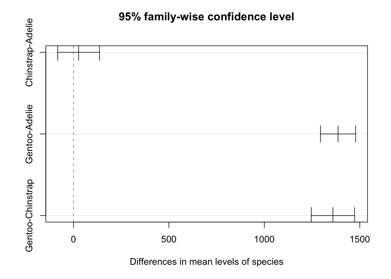
Interactions
In the previous example we assumed there were no interactions and so we had \(\gamma_{ij}=0\) for all \(i,j\). We will now relax this assumption and see what this could mean for the possible structure we can capture in data.
We can try to examine the relationship across each of the factors separately, but this could mask the connection to the other variable.

One way to examine the interaction between these factors is called an interaction plot, where we plot the average across each of the possible levels of the factors and see how these vary. This may not be perfect, but can give some insight into the relationship between the response and the two factors.

Looking at this interaction plot we see that how the average body mass changes from species to species does seem to be different within sex also. This is evidence that an interaction between these factors, given by \(\gamma_{ij}\neq 0\), might be required.
To fit the ANOVA model with an interaction we just need to include an interaction in the regression we fit initially.
int_fit <- lm(body_mass_g ~ species + sex + species * sex, data = penguins)

summary(int_fit)
Call:
lm(formula = body_mass_g ~ species + sex + species * sex, data = penguins)

Residuals:
    Min      1Q  Median      3Q     Max
-827.21 -213.97   11.03  206.51  861.03

Coefficients:
                         Estimate Std. Error t value Pr(>|t|)
(Intercept)               3368.84      36.21  93.030  < 2e-16 ***
speciesChinstrap           158.37      64.24   2.465  0.01420 *
speciesGentoo             1310.91      54.42  24.088  < 2e-16 ***
sexmale                    674.66      51.21  13.174  < 2e-16 ***
speciesChinstrap:sexmale  -262.89      90.85  -2.894  0.00406 **
speciesGentoo:sexmale      130.44      76.44   1.706  0.08886 .
---
Signif. codes:  0 '***' 0.001 '**' 0.01 '*' 0.05 '.' 0.1 ' ' 1

Residual standard error: 309.4 on 327 degrees of freedom
  (11 observations deleted due to missingness)
Multiple R-squared:  0.8546,    Adjusted R-squared:  0.8524
F-statistic: 384.3 on 5 and 327 DF,  p-value: < 2.2e-16
Now we have \(I\times J\) parameters to estimate, which again we can interpret. We need to check the residuals for this model. Note that if we want to estimate the standard deviation of the residuals this will be given by
\[ \hat{\sigma}_e =\sqrt{\frac{SSError}{n_{T}- IJ}}. \]
hist(int_fit$residuals)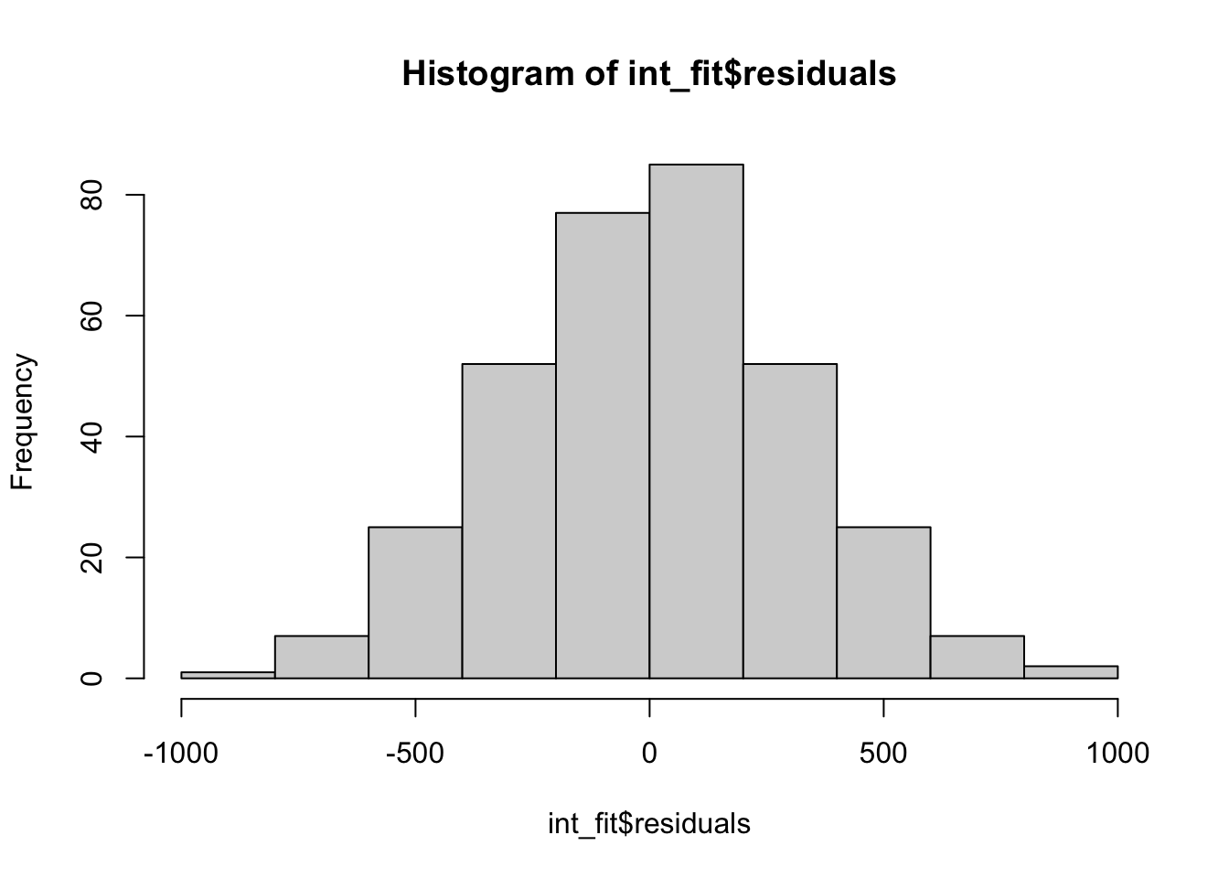
plot(x = int_fit$fitted.values, y = int_fit$residuals)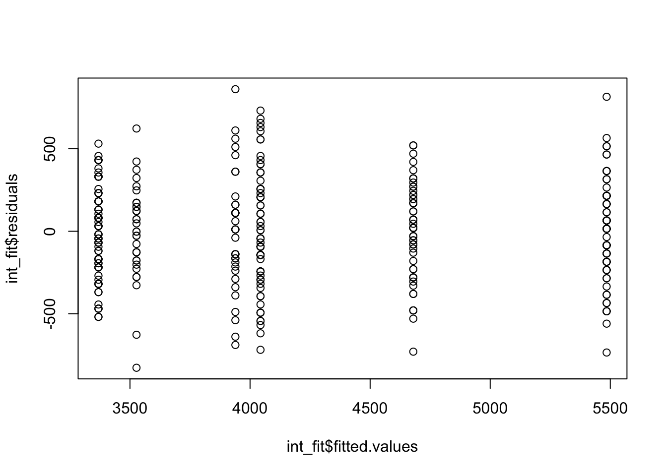
qqnorm(int_fit$residuals)
qqline(int_fit$residuals, col = "red")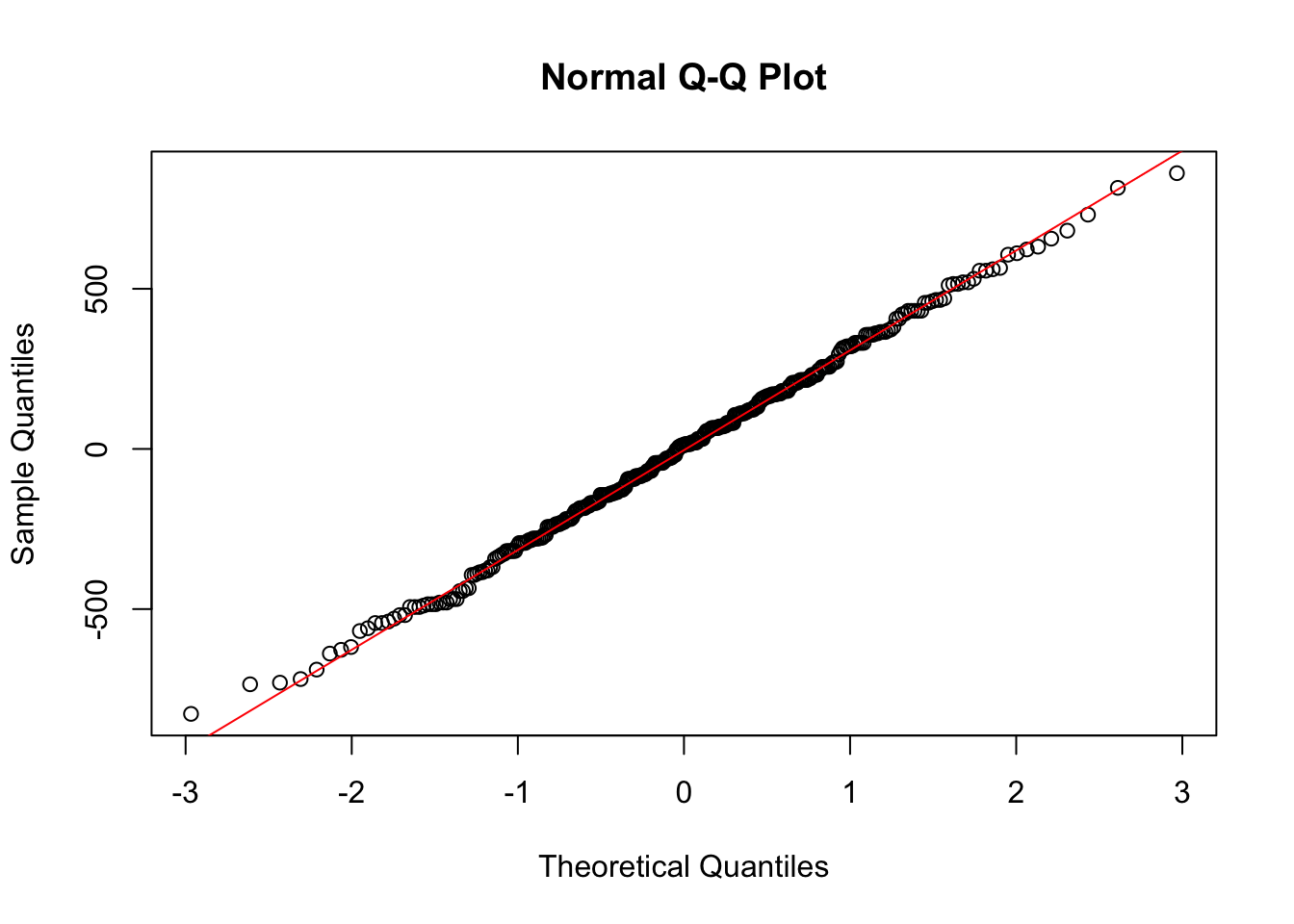
Looking at the residuals we see no problems, indicating no reasons to not believe that this two-way ANOVA with interactions is appropriate for this data. We can then construct the ANOVA table.
anova(int_fit)Analysis of Variance Table
Response: body_mass_g
Df Sum Sq Mean Sq F value Pr(>F)
species 2 145190219 72595110 758.358 < 2.2e-16 ***
sex 1 37090262 37090262 387.460 < 2.2e-16 ***
species:sex 2 1676557 838278 8.757 0.0001973 ***
Residuals 327 31302628 95727
---
Signif. codes: 0 '***' 0.001 '**' 0.01 '*' 0.05 '.' 0.1 ' ' 1Now we have an additional line, corresponding to the amount of the model sum of squares which is associated with the interaction effect, so we can write
\[ SSModel = SSA + SSB + SSAB. \]
There is an additional hypothesis test, corresponding to the presence of an interaction effect. This test is given by:
- \(H_0: \gamma_{ij}=0\) for all \(i,j\) vs the alternative, that at least one \(\gamma_{ij}\neq 0\), at some significance level.
We need to examine these hypotheses differently now when we have an interaction effect in the model. If you have an interaction then you should test this first, and we can do this test directly at significance level \(\alpha\).
The test statistic is given by \[ f = \frac{MSAB}{MSError} = 8.757 \]
for this example. Under the null hypothesis this is from an F distribution, where the first degree of freedom is \((I-1)(J-1)=2\) for this example and the second is \(df_E\), which in this example is \(n_T-6\) because we now have to estimate 6 parameters in this model. We see the p-value for this test statistic is less than significance \(\alpha\), so we reject the null hypothesis that there is no interaction between these factors.
Now, if we have an interaction, we have 3 possible hypothesis tests. As we have multiple tests, we need to be aware of the family wise Type 1 error, and whether we will control it or not. When there are interactions in the model we have two possible approaches:
We can initially test if there is an interaction effect at significance level \(\alpha\). If there is evidence for an interaction effect then we report that. If we do not reject the null hypothesis of there being no interaction, then we can subsequently test if we have effects for each of the two factors. If we do these then family wise error will not be controlled and these test should be considered somewhat exploratory.
Alternatively, we could instead consider all 3 possible tests at significance \(\alpha/3\), which would control the family wise error. We could also use Tukey’s HSD confidence intervals as part of this, but again, these should be explanatory and may not have the desired confidence.
Unbalanced Data
If our data is not balanced, then we need to be even more careful about how we perform the hypothesis tests of ANOVA. If we test the interaction effect \(H_0:\gamma_{ij}=0\) for all \(i,j\), then this will not change if the data is unbalanced. However, tests of the main effects will differ. To see this, we will fit the same two-way ANOVA model, except, we will include species as the first factor one time and sex as the first factor the other time. It turns out that our data is actually not sufficiently balanced here, based on these two models differing.
fit_1 <- lm(body_mass_g ~ species + sex + species * sex, data = penguins)

fit_2 <- lm(body_mass_g ~ sex + species + sex * species, data = penguins)

anova(fit_1)
Analysis of Variance Table
Response: body_mass_g
Df Sum Sq Mean Sq F value Pr(>F)
species 2 145190219 72595110 758.358 < 2.2e-16 ***
sex 1 37090262 37090262 387.460 < 2.2e-16 ***
species:sex 2 1676557 838278 8.757 0.0001973 ***
Residuals 327 31302628 95727
---
Signif. codes: 0 '***' 0.001 '**' 0.01 '*' 0.05 '.' 0.1 ' ' 1anova(fit_2)Analysis of Variance Table
Response: body_mass_g
Df Sum Sq Mean Sq F value Pr(>F)
sex 1 38878897 38878897 406.145 < 2.2e-16 ***
species 2 143401584 71700792 749.016 < 2.2e-16 ***
sex:species 2 1676557 838278 8.757 0.0001973 ***
Residuals 327 31302628 95727
---
Signif. codes: 0 '***' 0.001 '**' 0.01 '*' 0.05 '.' 0.1 ' ' 1Note now that we get different test statistics for species and sex depending on their order in the regression model! Note also that the test statistic for the interaction is the same both ways. This is because, we should read this ANOVA table from top to bottom, meaning we should actually partition the model sum of squares as
\[ SSModel = SSA + SS(B|A) + SS(AB|A,B). \]
What this means is that the sum of squares that is attributed to the second factor (factor B) will depend on the first factor (factor A). This can make correct inference challenging. We will not discuss this further but note that if your data is not sufficiently balanced, testing for the main effects in two-way ANOVA can be difficult.
Overall F-Test
When we did one way ANOVA, the F-test given in summary was equivalent to the one given by the ANOVA table. However, when we consider an additional factor this is no longer the case. We can still use the F-test in summary, we just need to know what it can be used to test.
In a general two-way ANOVA model then the corresponding F-test is that there are no effects, and the mean is the same across all groupings of the two factors.
\[ Y_{ijk} = \mu +\epsilon_{ijk}, \]
which means \(\alpha_1=\alpha_2=\ldots=\alpha_I = \beta_1 =\beta_2=\ldots = \beta_J = \gamma_{11} = \ldots = \gamma_{IJ} =0\). A small p-value indicates evidence to reject this hypothesis.
4.4 ANOVA for Regression
Previously when we used ANOVA with regression, we were somewhat limited by what we could test. We could only consider tests which checked if everything except \(\beta_0\) was zero on not. We can actually consider different tests, allowing us to test a subset of the coefficients as needed. This is known as a nested F-test. Once we know how to use the anova function, it is relatively straightforward to set up these tests in R.
Recall that when we looked at including binary and categorical predictors in regression we considered a model for the penguin data where both the slope and intercept could differ between male and female penguins. This gave us a linear regression model of the form
\[ Y =\beta_0 + \beta_1 X_1 +\beta_2 X_2 + \beta_3 X_1 X_2 + \epsilon. \]
Here, \(X_1\) is flipper length and \(X_2\) is an indicator variable, indicating sex is female (\(X_2=0\)) or male (\(X_2 =1\)). Before, we could either test whether each \(\beta=0\) individually, using a t-test, or we could test if \(\beta_1=\beta_2=\beta_3 =0\) using the standard F-test output in summary. Now we will see how we can use ANOVA to test a subset, such as
\[ H_0: \beta_2=\beta_3 = 0 \]
vs the alternative that at least one of \(\beta_2,\beta_3\neq 0\) at some significance level \(\alpha\). Testing if both of these coefficients are zero at once allows us to investigate whether there is evidence for a different regression line between species, where these lines could have a different slope or a different intercept, or both. This makes this a more general test than just looking at one of the coefficients on its own.
We will call the model when \(H_0\) is true the reduced model and when \(H_0\) is not true we will call the regression model the full model.
The test statistic for this test is then given by
\[ f = \frac{(SSModel_{A} - SSModel_{0})/d}{MSError_{A}}, \]
where \(SSModel_0\) is the model sum of squares under the reduced model and \(SSModel_A\) is the model sum of squares under the full model. \(d\) is the number of \(\beta\) coefficients we are testing, i.e how many parameters are in the full model which are zero in the null model. Finally, \(MSError_A\) is the Mean Squared Error under the full model.
To do this test, we need to pass the two regression fits to the ANOVA function. We will do this for the penguin data.
penguin_data <- na.omit(penguins)

fit1 <- lm(body_mass_g ~ flipper_length_mm, data = penguin_data)

fit2 <- lm(body_mass_g ~ flipper_length_mm + sex + flipper_length_mm * sex,
           data = penguin_data)

anova(fit1, fit2)
Analysis of Variance Table
Model 1: body_mass_g ~ flipper_length_mm
Model 2: body_mass_g ~ flipper_length_mm + sex + flipper_length_mm * sex
Res.Df RSS Df Sum of Sq F Pr(>F)
1 331 51211963
2 329 41794088 2 9417875 37.068 3.032e-15 ***
---
Signif. codes: 0 '***' 0.001 '**' 0.01 '*' 0.05 '.' 0.1 ' ' 1Now this \(F\) statistic is the one we want, and, under the null hypothesis, this comes from an \(F\)-distribution with \(d,df_{A}\) degrees of freedom. Here \(df_A\) is the number observations less the number of parameters we need to estimate under the full model. As the \(p\)-value is smaller than \(\alpha= 0.01\), for example, we have evidence to reject the null and conclude there is a different relationship between body mass and flipper length for the different sexes, which could be a different intercept or different slope, or both.
4.5 ANCOVA
Finally, we will talk briefly about one further extension of ANOVA, where we want to use ANOVA but we believe there is some other numeric predictor which may have a relationship with the outcome of interest. The general philosophy in statistics is that if there is a variable which affects the outcome of interest, you should account for this by including it in your model. This variable is often called a nuisance variable. In regression, we can do this by simply ensuring that we use that variable as a predictor. Now we want to see how to add a numeric predictor into an ANOVA model. This is known as analysis of covariance (ANCOVA). Here we will only see the one-way ANCOVA model and how to use it for an example.
The one-way ANCOVA model is given by
\[ Y_{ij} = \mu + \alpha_j + \beta X_{ij} + \epsilon_{ij}. \]
We are back to the notation of a one-way ANOVA model, so \(j\) is the group and \(i\) is the observation in a group. Now we have an overall global mean \(\mu\), and group level effects \(\alpha_j\) for \(i=1,2,\ldots,I\). For each observation we observe a numeric covariate that we believe will influence the relationship, so we want to include it in the model. We will assume here that the slope \(\beta\) for this covariate is the same across all the groups. We are interested in testing if the factor effects differ across groups. If we restrict \(\alpha_1=0\) then we are doing the following test.
- \(H_0:\alpha_1=\alpha_2=\ldots = \alpha_I=0\) vs \(H_A\), at least one \(\alpha_j\neq 0\) at some significance level \(\alpha\).
If this model feels a lot like fitting different intercepts for different categories of a predictor, that’s because it’s basically the same thing. ANCOVA just gives us a nice way of testing the \(\alpha\) effects being 0.
To use an ANCOVA model we need to check some conditions
- All the checks on an ANOVA model of \(Y\) and the factor of interest look ok
- All the checks on a regression between \(Y\) and \(X\) look ok
- There is no interaction between the factor variable and \(X\)
If we verify these conditions then we can fit our ANCOVA model. We first check the ANOVA model.
anova_fit <- lm(body_mass_g ~ species, data = penguins)
hist(anova_fit$residuals)
plot(anova_fit$fitted.values, anova_fit$residuals)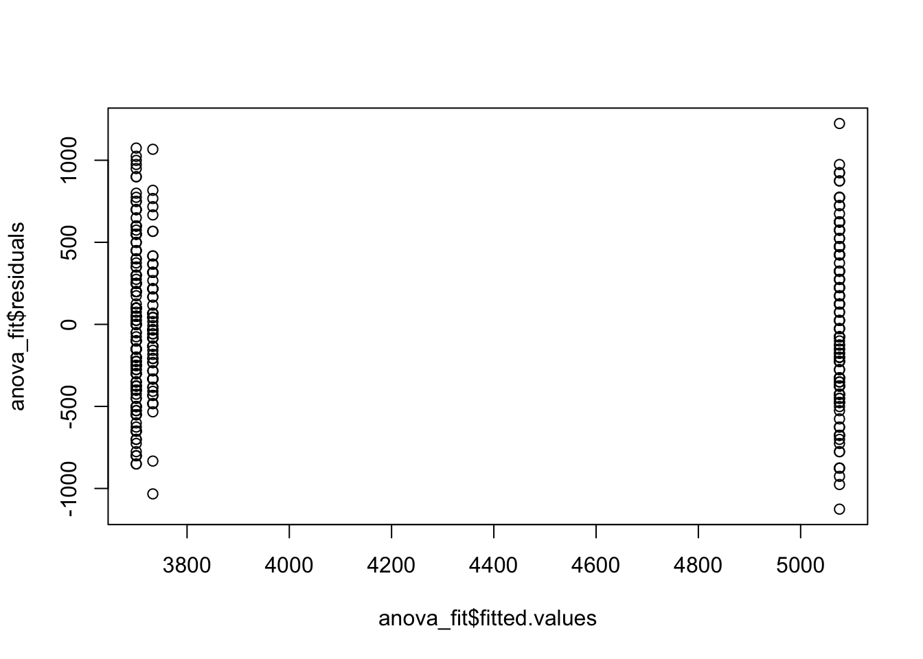
qqnorm(anova_fit$residuals)
qqline(anova_fit$residuals, col = "red")
Then, we can check the regression model.
reg_fit <- lm(body_mass_g ~ flipper_length_mm, data = penguins)
hist(reg_fit$residuals)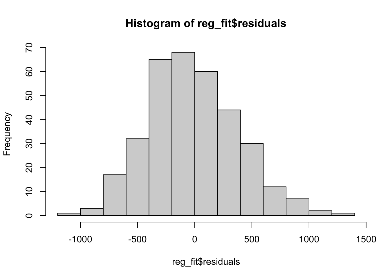
plot(reg_fit$fitted.values, reg_fit$residuals)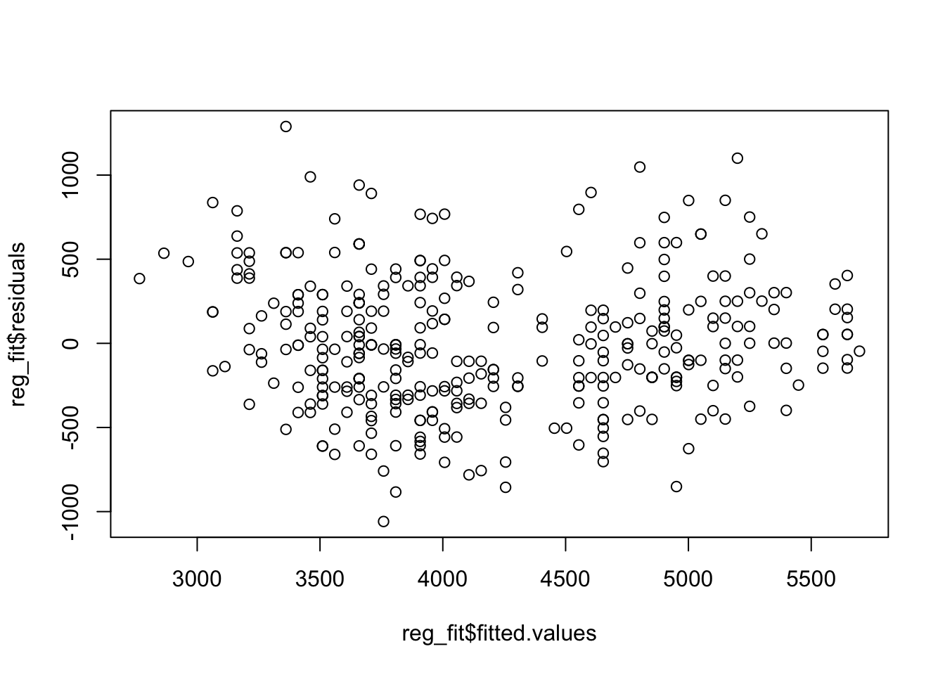
qqnorm(reg_fit$residuals)
qqline(reg_fit$residuals, col = "red")
Note that checking there is no interaction between the factor and \(X\) is equivalent to checking if there is a different slope across species. We will not check this here, and will assume this condition is ok, along with the others, allowing us to fit this model.
To fit this in R the numeric covariate should be the first term on the right hand side of lm. For the penguin data, we know that flipper length is highly correlated with body mass. So, if we are interested in seeing how body mass differs across sex, we should control for flipper length. The regression and ANCOVA table for this is shown below.
anc_fit <- lm(body_mass_g ~ flipper_length_mm + species, data = penguins)

anova(anc_fit)
Analysis of Variance Table
Response: body_mass_g
Df Sum Sq Mean Sq F value Pr(>F)
flipper_length_mm 1 166452902 166452902 1180.294 < 2.2e-16 ***
species 2 5187807 2593904 18.393 2.615e-08 ***
Residuals 338 47666988 141027
---
Signif. codes: 0 '***' 0.001 '**' 0.01 '*' 0.05 '.' 0.1 ' ' 1Then, the p-value given for species corresponds to testing if there is an effect of species, while controlling for flipper length. As this p-value is small, this is evidence to reject the null hypothesis and conclude there is a difference between species, at significance level \(\alpha\).
4.6 Summary and Examples
To recap, in this chapter on ANOVA we have seen:
- One-way ANOVA models and how you check the conditions for fitting such a model.
- Two-way ANOVA and the corresponding conditions for that
- How we can use ANOVA for testing a subset of coefficients in a regression model.
- ANCOVA, the conditions associated, and how we can use this to test the difference of means across groups in the presence of a nuisance continuous variable.
ANOVA is something of an extension of many of the regression methods we saw previously. In some ways, it allows you to examine more specific questions, and in different ways, to how you can do that using regression models. However, with these more flexible and (potentially) more powerful statistical tools comes with more challenges. We have more assumptions that need to be satisfied for ANOVA models to work. Both the benefits and challenges of ANOVA are important if you ever want to use it to analyse data!
To finish up this section we will see some more examples of how we can use ANOVA techniques to analyse data.
Example
We collect data about American Robins, some of whom have been treated with a hormone. We want to examine if there is an effect on the blood Calcium level of these Robins based on this hormone. We have both Male and Female Robins so we will use two-way ANOVA. To do this we should ask a few questions:
- Should we have an interaction effect in our model?
- Is our data balanced?
To check if it is balanced we can just see how many observations are in each level of the two factors.
# A tibble: 4 × 3
# Groups:   Sex [2]
  Sex    Hormone     n
  <fct>  <fct>   <int>
1 female no          5
2 female yes         5
3 male   no          5
4 male   yes         5
As we have the same (small!) number of birds in each group, our data is balanced. We will do an interaction plot to see if there is evidence for an interaction between Sex and Hormone.
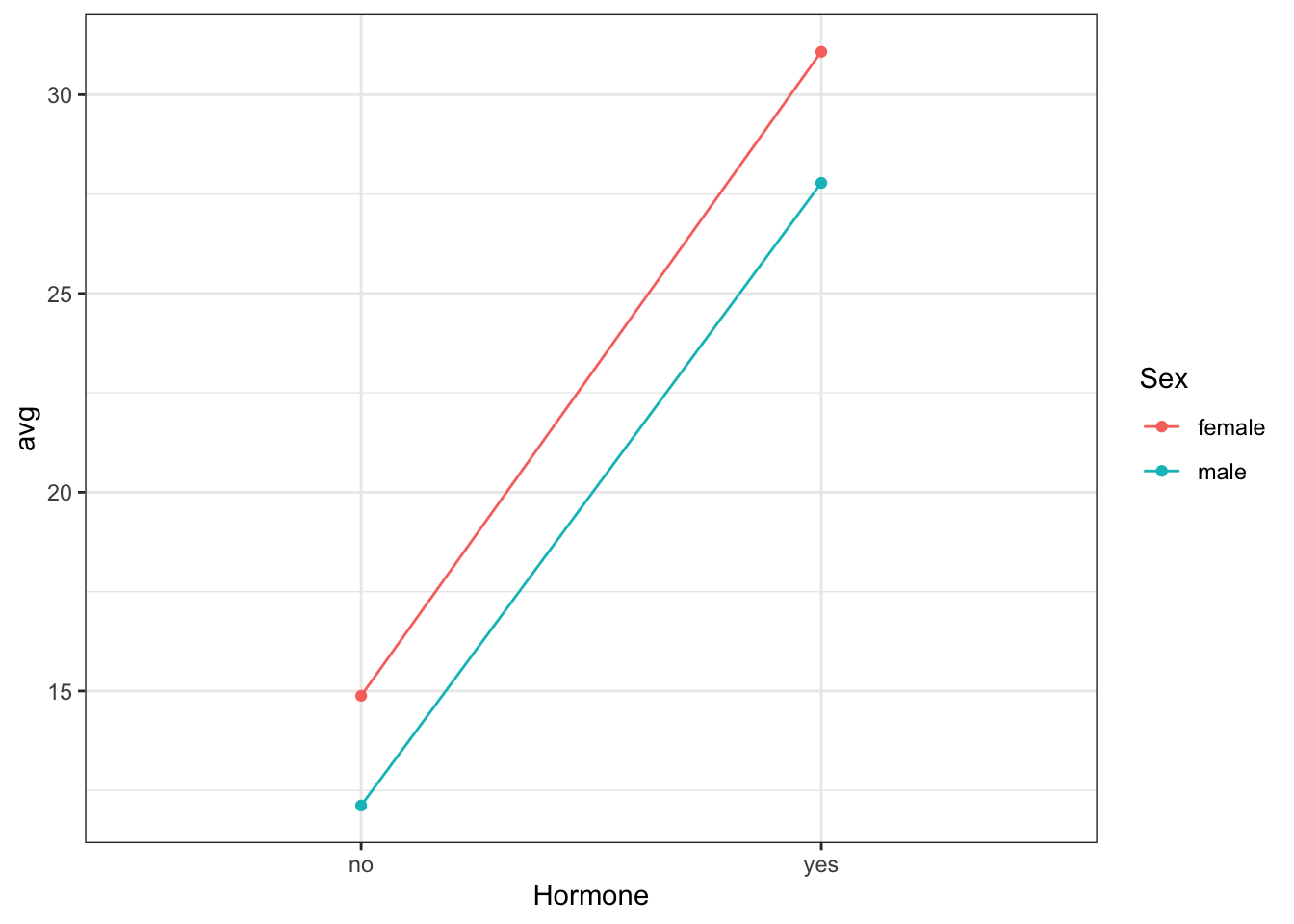
These lines appear to be almost parallel, indicating there is maybe not an interaction present. This is an informal way of deciding whether to include an interaction in our model. If you believe there is an interaction present then it should be included and tested, as described previously.
We will now fit this two way ANOVA model. We first need to check the conditions for the residuals.
reg_model <- lm(Ca ~ Sex + Hormone, data = BirdCalcium)

hist(reg_model$residuals)
plot(x = reg_model$fitted.values, y = reg_model$residuals)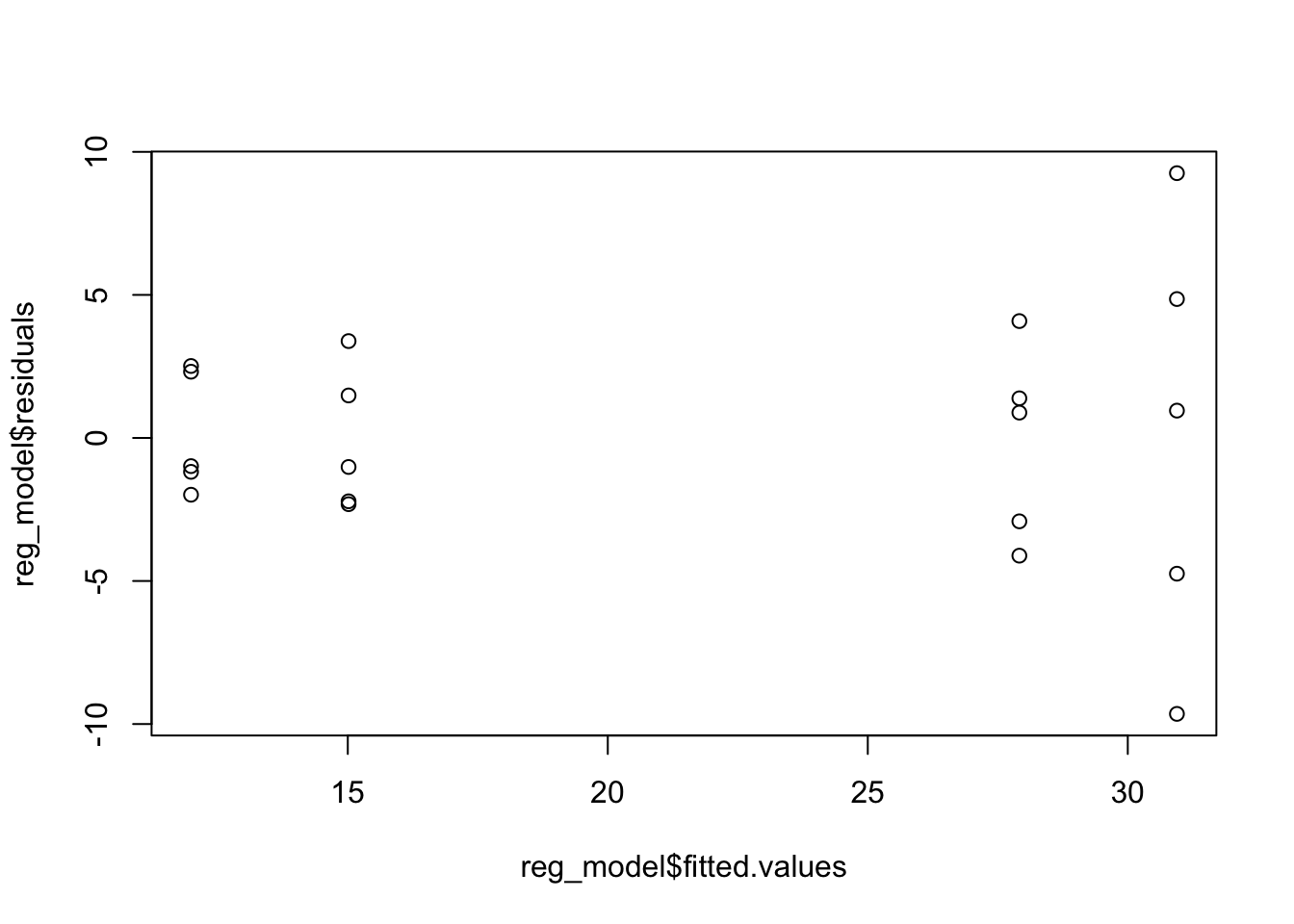
qqnorm(reg_model$residuals)
qqline(reg_model$residuals, col = "red")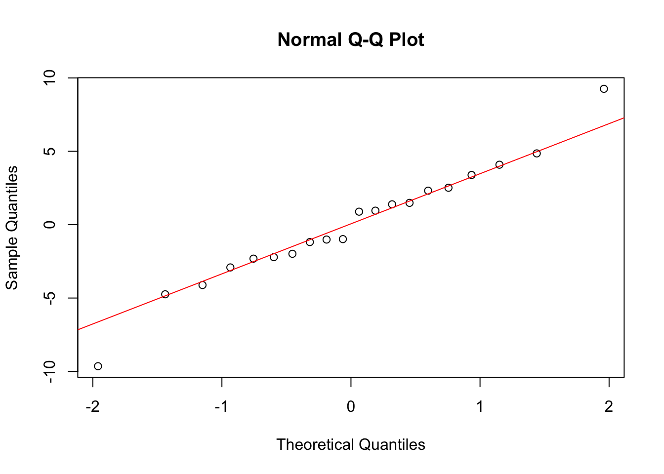
We don’t have too many observations here, but we can still look at these results and maybe be a little more careful about checking the assumptions. As these conditions look ok, we can construct the ANOVA table and interpret the output. We will consider significance level \(\alpha = 0.01\). Here we will need to compare the p-values after doing a Bonferroni correction.
anova(reg_model)Analysis of Variance Table
Response: Ca
Df Sum Sq Mean Sq F value Pr(>F)
Sex 1 45.90 45.90 2.4896 0.133
Hormone 1 1268.82 1268.82 68.8134 2.22e-07 ***
Residuals 17 313.46 18.44
---
Signif. codes: 0 '***' 0.001 '**' 0.01 '*' 0.05 '.' 0.1 ' ' 1Now, we see that we have evidence for an effect of Hormone on the blood Calcium level, at \(\alpha/2 = 0.005\). We do not have evidence for an effect of Sex here. We could then also look at the Tukey plots, however as there are only two levels (Hormone or Not), this will give a single confidence interval. This is further evidence for a difference in blood Calcium across the levels of the Hormone factor (whether a bird received the hormon or not).
tukey <- TukeyHSD(aov(reg_model), which = "Hormone", conf.level = 0.95)
plot(tukey)
Example
For another example, we will consider data on Horse prices, along with their Height and Sex. We want to see how appropriate an ANCOVA model is here, where we are interested in seeing if there is a difference in horse prices across sex, while controlling for the height of a horse.
To do this, we need to check the conditions required for one-way ANCOVA. For this we need to fit two models in lm and make sure both residuals look ok. Recall that the one-way ANCOVA model is given by
\[ Y_{ij} = \mu + \alpha_j + \beta X_{ij} + \epsilon_{ij}, \]
so the other assumption we need to check is whether a common slope (here for both male and female horses), between the response and the nuisance \(X\) variable, is ok. We will check this last condition visually first. Note that because price is a positive variable, we will take a log transformation of \(Y\).
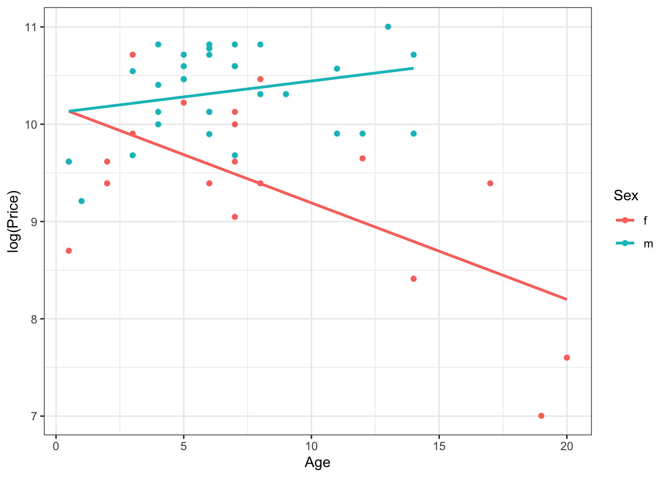
Here, we are fitting separate regression lines for both male and female horses. From this, it is pretty obvious that this condition for a one-way ANCOVA model is not satisfied, and therefore we can’t use one-way ANCOVA. If this was a real analysis and you see that one of the conditions is not satisfied, you can essentially conclude right away that an ANCOVA model won’t work. For the sake of completeness, we will check the other conditions here too.
We first need to fit a one-way ANOVA model (without the nuisance variable), and see if the assumptions for such a model are reasonable.
anova_check <- lm(log(Price) ~ Sex, data = HorsePrices)

hist(anova_check$residuals)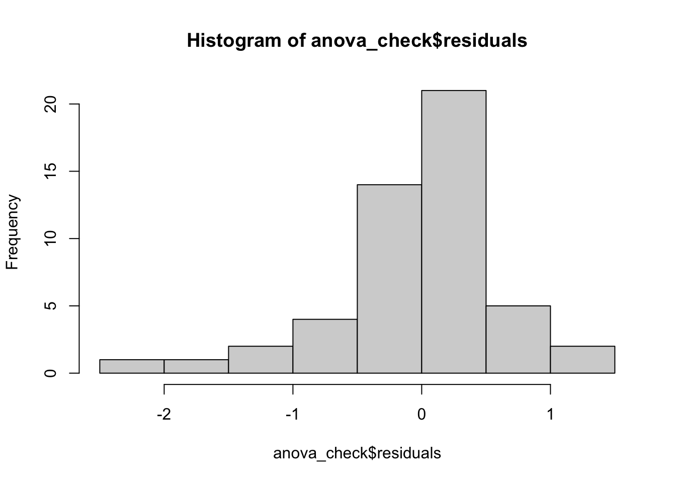
plot(x = anova_check$fitted.values, y = anova_check$residuals)
qqnorm(anova_check$residuals)
qqline(anova_check$residuals, col = "red")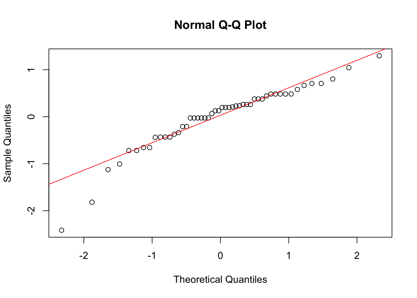
Here, we see from the histogram that the residuals are maybe not normally distributed with mean zero. Similarly, the spread of the residuals seems to differ across the two groups. Finally, the normal quantile plot, while looking somewhat ok, still has some concerning points.
We should already be certain that an ANCOVA model isn’t the right approach for this data, but we will still check the final set of assumptions. We fit a simple linear regression between the response and the nuisance variable and see if the assumptions for a regression model are met.
lm_fit <- lm(log(Price) ~ Height, data = HorsePrices)

hist(lm_fit$residuals)
plot(x = lm_fit$fitted.values, y = lm_fit$residuals)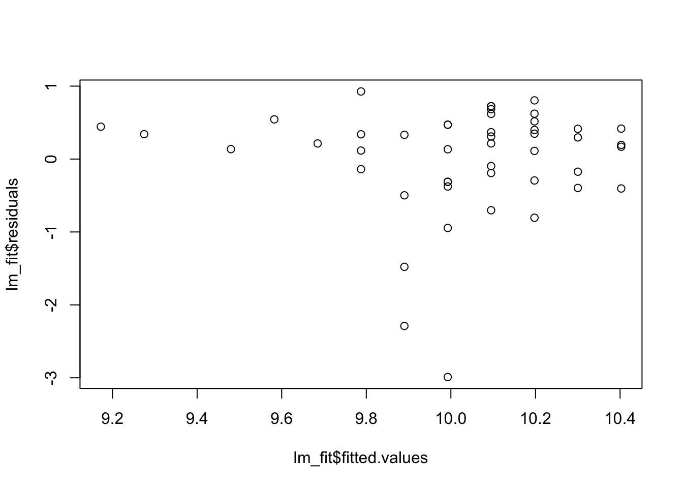
qqnorm(lm_fit$residuals)
qqline(lm_fit$residuals, col = "red")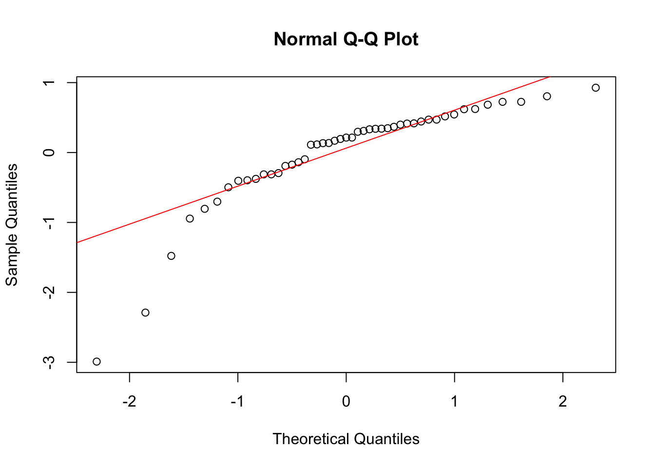
Now again, we see clear problems with these assumptions. Everything is saying a one-way ANCOVA model is not correct for this data. Remember though, that we need all three sets of assumptions we considered here to be reasonable to fit a one-way ANCOVA model.
Example
As a final example, lets consider a setting where we want to use the tools of ANOVA to test for a subset of regression coefficients. While we have previously used this to test for categorical predictors, that does not need to be the case. This example is based on one in Cannon et al. (2018). We will examine data about NFL teams in the 2016 season, and we are interested in seeing the role of team metrics in predicting the Win Percentage of a team in the regular season.
Before doing this problem, you might think that because a percentage is between 0 and 100, that a regression model, which allows the response to take on any possible real value, is not appropriate. However in practice, once you do not have percentage that are exactly 0 or 100% then a linear regression can work well for this data.
We will have two choices of model.
Model 1, the simpler model, where as predictors for win percentage we use the points a team concede (
PointsAgainst), the yards a team give up (YardsAgainst) and the number of touchdowns the team scores (TDs).Model 2, the full model, where we also include the number of points a yards a teams obtains in the season (
PointsForandYardsFor).
Now, we can write our regression model as
\[ Y = \beta_0 + \beta_1 X_1 + \beta_2 X_2 + \beta_3 X_3 + \beta_4 X_4 + \beta_5 X_5 + \epsilon, \]
where:
\(X_1\) is
PointsFor\(X_2\) is
PointsAgainst\(X_3\) is
YardsFor\(X_4\) is
YardsAgainst\(X_5\) is
TDs
and the test then becomes
\[ H_0: \beta_1 = \beta_3 = 0 \]
against the alternative that both \(\beta_1\) and \(\beta_3\) are not zero. We will test this at \(\alpha = 0.1\).
Note that for a nested F-test to be valid, we need to know that a regression model is appropriate for this data! We can check this using the regular tools for checking a (multivariate) regression model. For problems like this where you are comparing two regression models, we should make sure the assumptions are ok for both the potential models. These checks are not shown here but have been satisfied.
Given this, we can fit the two regression models and then use anova to get the test statistic for this hypothesis test.
data("NFLStandings2016")

full_model <- lm(WinPct ~ PointsFor + PointsAgainst + YardsFor +
                   YardsAgainst + TDs, data = NFLStandings2016)


reduced_model <- lm(WinPct ~ PointsAgainst + YardsAgainst +TDs, data = NFLStandings2016)

anova(reduced_model, full_model)
Analysis of Variance Table
Model 1: WinPct ~ PointsAgainst + YardsAgainst + TDs
Model 2: WinPct ~ PointsFor + PointsAgainst + YardsFor + YardsAgainst +
TDs
Res.Df RSS Df Sum of Sq F Pr(>F)
1 28 0.23831
2 26 0.22183 2 0.016481 0.9658 0.3939Here \(n=32\) for the 32 teams in the NFL so the test statistics comes from an F-distribution with \(2,26\) df, because we need to estimate 6 paramaeters in the full model. When we do this test we get a p-value larger than \(\alpha=0.1\), so we have no evidence to reject \(H_0\) at this significance level. Is this result surprising? That how many points a team scores, or yards they get, are not good predictors for the percentage of games they win?
If you know a bit about football, you might realise why this is the case. The reduced model includes TDs, the number of touchdowns a team scores. This will be highly correlated with both the number of points they score, and the number of yards they get. So it is unsurprising that if we add a correlated predictor it is not significant. If you remember how we identified correlated predictors in the past, we can look at the vif scores of the full model.
library(car)
vif(full_model)
PointsFor PointsAgainst YardsFor YardsAgainst TDs
20.788183 1.804447 3.916398 1.888166 16.471121 Now we get large VIF scores, indicating these predictors are highly correlated. This helps us make sense of the result of our hypothesis test.