# A tibble: 6 × 3
   diam height volume
  <dbl>  <dbl>  <dbl>
1   8.3     70   10.3
2   8.6     65   10.3
3   8.8     63   10.2
4  10.5     72   16.4
5  10.7     81   18.8
6 10.8 83 19.73 Multiple Linear Regression
3.1 Introduction
So far we have spent quite a bit of time understanding how linear regression works when we observe two variables, \(X\) and \(Y\), and we have \(X\) as our explanatory variable and \(Y\) as our response variable.
However, in many of these examples, we could in fact have recorded data for more than two variables. For example, for the cherry tree data we had volume as our response and diameter as the explanatory variable. This dataset actually contained another variable, the height of a tree.
Would this also make sense to include in our model? You might think that both these variables (height and diameter) would be important in understanding the volume of a tree, and so we would like to use both in our statistical model.
We can actually include two (or even more) explanatory variables in our model. Things get slightly more complicated than the previous setting, but most of the ideas we have seen before can be extended to allow this. However, when we have many variables there can be problems and it becomes much harder to understand the relationship between these variables and our response. The simple nature of the relationship when we only have one predictor variable is one of the big benefits of a simple linear regression model.
Similarly, even if we have many variables we could use in our model, it might not actually make sense to include them all, and an important task is identifying which variables are most “important”. We will see how to consider each of these problems later, but first we can consider a slightly different setting, somewhat similar to the transformations we saw before.
3.2 Polynomial Regression
Before we consider adding multiple explanatory variables, we can instead consider ways to capture non linear patterns.
Remember that a linear regression is of the form
\[ Y = \beta_0 + \beta_1 X +\epsilon \]
However, we could also include \(X^2\) in our model. Then we could write
\[ Y= \beta_0 + \beta_1 X +\beta_2 X^2 + \epsilon \]
A natural question to ask is whether this is a linear regression or not. It turns out that it is still a linear regression, because it is linear in the coefficients, which are \(\beta_0, \beta_1, \beta_2\). We are just taking non linear functions of the \(x\) variable, not of these coefficients.
We could also have tried the model
\[ Y_i = \beta_0 + \beta_1 \cos(X_i) + \beta_2 \sin(X_i) +\epsilon_i, \]
which is also a linear regression. For a model to be linear, we just need:
- The parameters/coefficients, the \(\beta\) terms, to be linear
- The errors, \(\epsilon\), to have mean 0
We will only consider polynomial regression here but much more complex models can be used too, which are beyond the scope of this class.
A polynomial regression model of order p is given by the equation
\[ Y = \beta_0 + \beta_1 X + \beta_2 X^2 + \ldots + \beta_p X^p + \epsilon. \]
Here we could have \(p=1\), which is the standard linear regression model we saw before, or a larger value of \(p\). We will still make the same assumptions that the data \((x_i, y_i)\) are all independent and that the errors \(\epsilon_i\) all come from a normal distribution with fixed variance \(\sigma^2\), and are all independent. We call p the degree of the polynomial.
Example
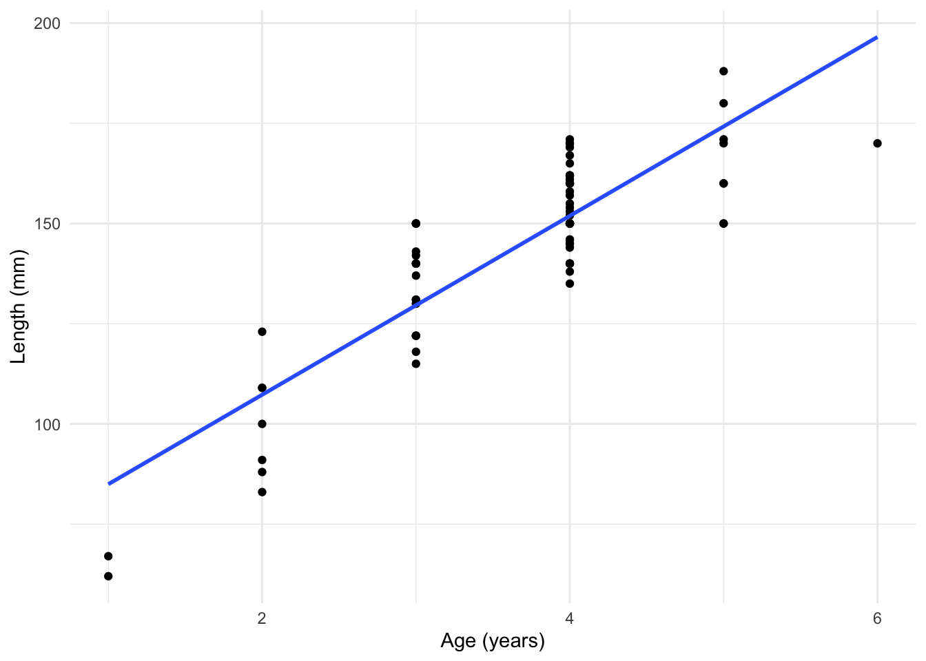
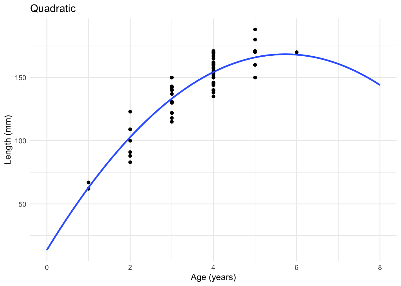
To see this, lets consider a simple example. We collect a sample of fish and record their age and their length. Fitting a regular linear regression is not that appropriate for the type of data we have here, as can be seen below.
Fitting a Polynomial Model
We can actually fit this model in a very similar way to the original regression model. Just as importantly, we can use very similar R code to fit it in practice. For this example, we fit a quadratic model, so that
\[ Y = \beta_0 + \beta_1 X + \beta_2 X^2 + \epsilon. \]
We can fit this in R using the lm function once again. We need to make the use of age^2 as a separate covariate explicit here, and one way to do this is through the use of I around it. This gives us the same output as before, except now we get an additional row, corresponding to information about \(\hat{\beta}_2\), the estimate of the coefficient of \(X^2\).
fit_quad <- lm(length ~ age + I(age^2), data = fish_data)

summary(fit_quad)
Call:
lm(formula = length ~ age + I(age^2), data = fish_data)
Residuals:
Min 1Q Median 3Q Max
-19.846 -8.321 -1.137 6.698 22.098
Coefficients:
Estimate Std. Error t value Pr(>|t|)
(Intercept) 13.622 11.016 1.237 0.22
age 54.049 6.489 8.330 2.81e-12 ***
I(age^2) -4.719 0.944 -4.999 3.67e-06 ***
---
Signif. codes: 0 '***' 0.001 '**' 0.01 '*' 0.05 '.' 0.1 ' ' 1
Residual standard error: 10.91 on 75 degrees of freedom
Multiple R-squared: 0.8011, Adjusted R-squared: 0.7958
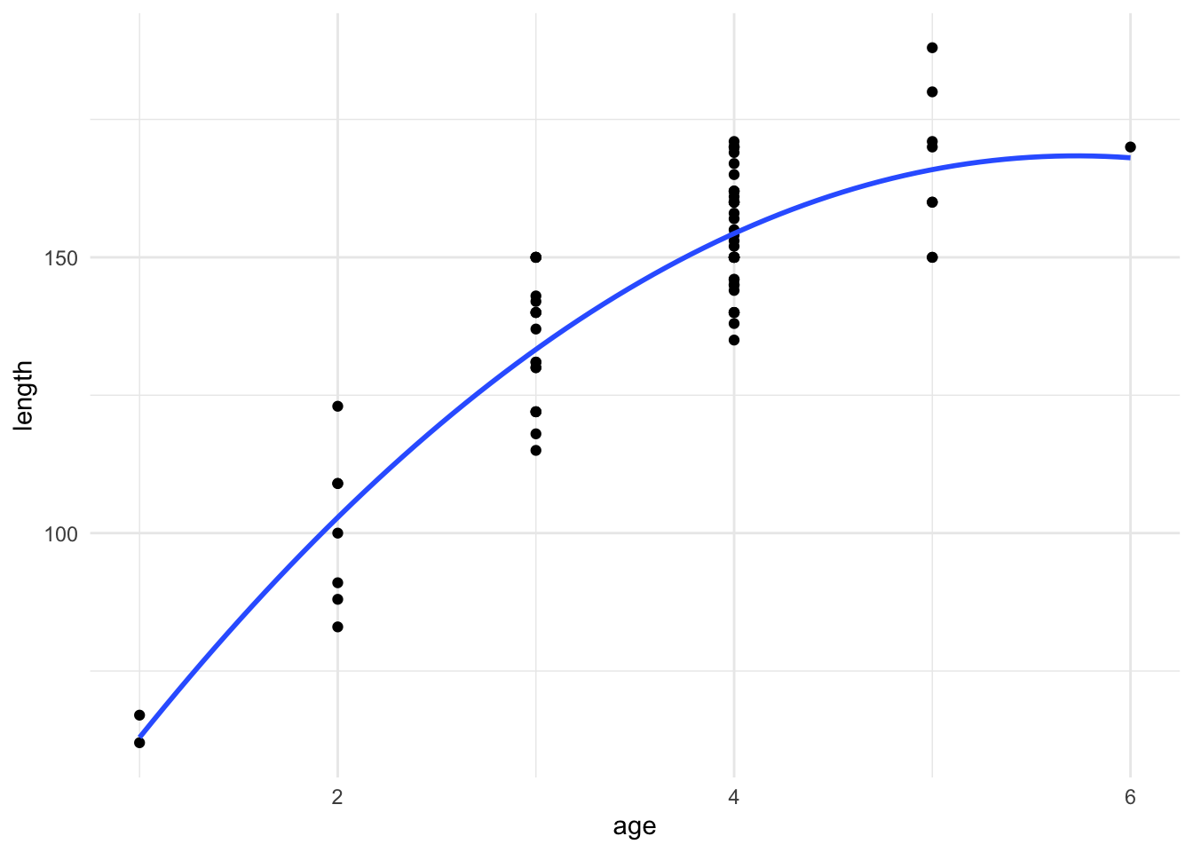
F-statistic: 151.1 on 2 and 75 DF, p-value: < 2.2e-16We can then plot this fitted model, and we see that this quadratic function seems to describe the data better than a simple straight line.
As before, we need to check the assumptions of our regression model before we interpret our results. These are the same assumptions as we saw for the simpler setting, and we can use the same R code to construct the plots.
Remember that we want to check:
- That the data is independent.
- That the residuals are normally distributed with mean 0, and some fixed variance which does not change as \(x\) changes.
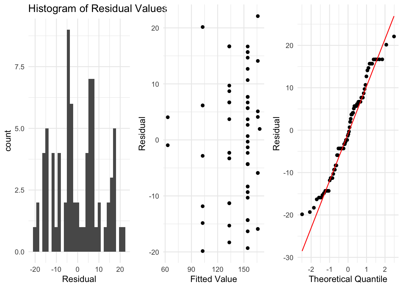
These residuals look somewhat reasonable for this example now, and there are no clear problems which we should be worried about. So for this example, we can conclude the quadratic model is probably ok and we can move on to interpreting the output of the model.
Inference for a Polynomial Model
Given that we have fit a polynomial regression and decided it’s an appropriate model for our data, we can then interpret that model and investigate the estimated parameters, in much the same way we did this previously.
F-test for all slope coefficients \(=0\)
This is the first place where we can see how the ANOVA method we saw before gives us something different to the regular t test. Now we can use it to test something more complicated. For example, our proposed polynomial regression model is
\[ Y = \beta_0 + \beta_1 X + \beta_2 X^2 + \epsilon, \]
and now the F test can be used to test:
- \(H_0:\) That \(\beta_1 =\beta_2 = 0\)
- \(H_A:\) That at least one of \(\beta_1,\beta_2\neq 0\),
at some significance level \(\alpha\).
Recall that when we do a hypothesis test like this we look at the sums of squares in the model, and our test statistic is given by
\[ f = \frac{MSModel}{MSError}, \]
Where \(MSModel = SSModel/df_{M}\), with \(df_M\) the degrees of freedom of the model. This was 1 in Chapter 2 but will change now, depending on the order of the polynomial. Remember that
\[ SSTotal = SSModel + SSError, \]
and \(SSTotal\) has \(n-1\) degree of freedom, because we just estimate \(\bar{y}\). Now \(SSError\) has \(n-p-1\) degrees of freedom, because under the polynomial model of order \(p\), we estimate \(p+1\) parameters, \(\beta_0,\beta_1,\ldots, \beta_p\). Therefore the model term will have \(p\) degrees of freedom, and under the null hypothesis, \(f\) comes from an \(F\) distribution with \(p,n-p-1\) degrees of freedom, \(F_{p,n-p-1}\). The \(F\) distribution can only take on positive values, and we reject the null hypothesis if \(f\) is either very small (just above 0) or very large. As before we can compute explicit critical values for an \(F\) distribution, using df however now they are not symmetric and so qf(0.025, df1 = 1, df2 = 10, lower.tail = TRUE) and qf(0.025, df1 = 1, df2 = 10, lower.tail = FALSE) will not be related.
qf(0.025, df1 = 2, df2 = 75, lower.tail = TRUE)[1] 0.02532636qf(0.025, df1 = 2, df2 = 75, lower.tail = FALSE)[1] 3.876416In practice, it is convenient to just look at the \(p\)-value given in the output. For this example we have \(p=2\), and we can examine the \(p\)-value given in the summary output to decide whether to reject or fail to reject our null hypothesis.
summary(fit_quad)
Call:
lm(formula = length ~ age + I(age^2), data = fish_data)

Residuals:
    Min      1Q  Median      3Q     Max
-19.846  -8.321  -1.137   6.698  22.098

Coefficients:
            Estimate Std. Error t value Pr(>|t|)
(Intercept)   13.622     11.016   1.237     0.22
age           54.049      6.489   8.330 2.81e-12 ***
I(age^2)      -4.719      0.944  -4.999 3.67e-06 ***
---
Signif. codes:  0 '***' 0.001 '**' 0.01 '*' 0.05 '.' 0.1 ' ' 1

Residual standard error: 10.91 on 75 degrees of freedom
Multiple R-squared:  0.8011,    Adjusted R-squared:  0.7958
F-statistic: 151.1 on 2 and 75 DF,  p-value: < 2.2e-16
For this test at \(\alpha = 0.05\), because this \(p\)-value is smaller than \(\alpha\), we reject the null hypothesis that \(\beta_1=\beta_2=0\) at \(\alpha =0.05\).
Test if highest order term is 0
While the previous section described how to test if any coefficients of \(X\) are statistically different from 0, perhaps more interesting would be understanding whether the highest order term is 0 or not. For example, if you fit a quadratic model,
\[ Y = \beta_0 +\beta_1 X + \beta_2 X^2 +\epsilon, \]
you might be interested in testing whether you need the quadratic \(X^2\) term, or if a standard linear regression (\(\beta_2=0\)) is sufficient.
We want to test if \(H_0:\beta_2 = 0\) vs \(H_A:\beta_2\neq 0\) at significance level \(\alpha\). We can do this in the exact same way as before. The test statistic is given by
\[ t = \frac{\hat{\beta}_2 - 0}{se(\hat{\beta}_2)}, \]
where we can get this test statistic and each term in it from summary. Under the null hypothesis that \(\beta_2 = 0\), then \(t\) follows a t distribution with \(n-p-1\) degrees of freedom. As before, we get the p-value for this test for free from the output of summary.
We can also construct a confidence interval for \(\beta_2\), using the standard error in the output and looking up the corresponding t-score needed, with \(n-p-1\) degrees of freedom.
For this example we can see that the output tells us that a hypothesis test for \(\beta_2=0\) at \(\alpha = 0.01\) (for example) would reject the null hypothesis of this coefficient being zero.
We can do the same procedure for other coefficients, such as \(\beta_1\), however this is conditional on \(\beta_0\) and \(\beta_2\) being in the model.
How to choose p?
An important question when considering these polynomial models is the choice of \(p\). Why should we use \(p=2\) instead of \(p=4\), or even \(p=8\)?
Note that the \(F\) test will still test if all coefficients are zero or not, but it can become hard to determine how many coefficients you actually need. Using the \(p\)-values from summary also has potential problems. We will not go into in detail here, but essentially doing many t-tests (i.e, looking at all the \(p\)-values for each coefficient), can lead to major problems with your analysis.
Similarly, when you add more polynomials to your model, you make it more complicated, and it can lead to overfitting. Lets see this with an example. We will look at opinion poll data up to the democratic convention in the US in 2016 for two of the main candidates, Clinton and Sanders. We are interested in predicting how the opinion poll results will look for the following months. While you might have some (valid) concerns about using a regression model for time series data like this, it can often work well.

We will consider two potential models here:
A simple linear regression \(Y =\beta_0 + \beta_1 X + \epsilon\), where \(X\) is the date and \(Y\) is the share of the vote Clinton or Sanders receives.
A polynomial regression of order \(5\), given by \(Y = \beta_0 + \beta_1 X + \beta_2 X^2 +\beta_3 X^3 + \beta_4 X^4 +\beta_5 X^5 +\epsilon\), for the same \(X\) and \(Y\).
We can fit both of these models to this data.


When we look at the output of this fifth order polynomial model, the F test indicates that the hypothesis of all coefficients of \(X\) being 0 is rejected and several of the \(\beta\) coefficients are statistically significant.
## poly also fits a polynomial regression
summary(lm(Clinton ~ poly(Date,5), data = realclear[train, ]))
Call:
lm(formula = Clinton ~ poly(Date, 5), data = realclear[train,
    ])

Residuals:
     Min       1Q   Median       3Q      Max
-17.8003  -3.1189   0.3729   3.7856  20.4931

Coefficients:
               Estimate Std. Error t value Pr(>|t|)
(Intercept)     57.0902     0.5333 107.059  < 2e-16 ***
poly(Date, 5)1 -49.8509     5.8900  -8.464 9.09e-14 ***
poly(Date, 5)2 -29.2684     5.8900  -4.969 2.34e-06 ***
poly(Date, 5)3   9.7054     5.8900   1.648  0.10211
poly(Date, 5)4  17.3707     5.8900   2.949  0.00385 **
poly(Date, 5)5  15.2980     5.8900   2.597  0.01061 *
---
Signif. codes:  0 '***' 0.001 '**' 0.01 '*' 0.05 '.' 0.1 ' ' 1

Residual standard error: 5.89 on 116 degrees of freedom
Multiple R-squared:  0.4967,    Adjusted R-squared:  0.475
F-statistic:  22.9 on 5 and 116 DF,  p-value: 6.253e-16
Which model would you suspect will do better at predicting the opinion polls in the next month? It appears that the polynomial model captures some trends in the data better than the simple regression model.
We can then show the next few opinion polls, along with the predictions from these two models.

The polynomial model overfits to the original data and is then not able to give good predictions for the new opinion polls. This means that it tries to make the model it fits match the data very closely (as it is a flexible model). If it turned out that the true model didn’t match the fitted model, this can lead to large errors, as we see here. Meanwhile, the simple regression model, while appearing to not fit the data as well, is actually more suited for making predictions for new data. This is because it cannot match the data in 2015 as closely.
It is quite common that more complicated models can appear to be better but when we actually evaluate them properly, such as for making predictions for new data, a less complex model can be more effective and also easier to understand. This is important to keep in mind as we continue looking at more complicated models.
Confidence Intervals for \(y\)
Much like the previous regression setting, we can also get confidence and prediction intervals for \(y\) at a new data point \(x_{new}\). The formulas for the standard errors are not shown here. The prediction intervals will be wider than the confidence intervals, by the same logic as we saw previously. For example, we can easily get 90% confidence and prediction intervals for \(x_{new}=4\). Because \(x_{new}^2\) can be computed directly from \(x_{new}\), you only need to specify the \(x\) variable, i.e the same variables we specified in the original fit of the model.
new_x <- data.frame(age = 4)
predict(fit_quad, newdata = new_x, interval = "confidence", level = 0.9)
fit lwr upr
1 154.321 151.9609 156.681predict(fit_quad, newdata = new_x, interval = "prediction", level = 0.9) fit lwr upr
1 154.321 136.005 172.6369While this is all the time we will spend on polynomial regression models, the next version we consider, with multiple predictors, has many similarities.
3.3 Two Explanatory Variables
Much like the polynomial regression model, we can have two rather than one predictor variables in our model. Let’s consider this for the tree data, using the model
\[ Y = \beta_0 +\beta_1 X_1 + \beta_2 X_2 +\epsilon \]
For this example \(Y\) is the volume of a tree, \(X_1\) is the diameter and \(X_2\) is the height. That is, for tree \(i\) we observe the volume \(Y_i\), the diameter \(X_{{1}i}\) and the height \(X_{2i}\). We observe variables \(X_1\) and \(X_2\) for each row in our data. This is a linear regression and so we fit and check the conditions in the same way we did for our original regression models. However, we again need to be careful interpreting the terms in our model.
reg_fit <- lm(volume ~ diam + height, data = tree_data)

summary(reg_fit)
Call:
lm(formula = volume ~ diam + height, data = tree_data)

Residuals:
    Min      1Q  Median      3Q     Max
-6.4065 -2.6493 -0.2876  2.2003  8.4847

Coefficients:
            Estimate Std. Error t value Pr(>|t|)
(Intercept) -57.9877     8.6382  -6.713 2.75e-07 ***
diam          4.7082     0.2643  17.816  < 2e-16 ***
height        0.3393     0.1302   2.607   0.0145 *
---
Signif. codes:  0 '***' 0.001 '**' 0.01 '*' 0.05 '.' 0.1 ' ' 1

Residual standard error: 3.882 on 28 degrees of freedom
Multiple R-squared:  0.948, Adjusted R-squared:  0.9442
F-statistic:   255 on 2 and 28 DF,  p-value: < 2.2e-16
We can check the conditions for this regression model, by looking at the residuals, in the same way we did this before.

Here the residuals look to satisfy the normality assumptions well, indicating we can go on and interpret the results of our model.
One important point to note is that when we have this model with \(X_1\) and \(X_2\), how the residual standard deviation is calculated changes slightly. The formula for it is now
\[ \hat{\sigma}_e = \sqrt{\frac{\sum_{i=1}^{n}(y_i - \hat{y}_i)^2}{n -2 -1}}. \]
Note that the denominator has changed. We have 2 predictors here, \(X_1\) and \(X_2\) but we could have more. If we had \(p\) predictors \(X_1,X_2,\ldots,X_p\) then the model would be
\[ Y = \beta_0 + \beta_1 X_1 + \beta_2 X_2 + \ldots + \beta_p X_p +\epsilon \]
and the residual standard deviation would be given by
\[ \hat{\sigma}_e = \sqrt{\frac{\sum_{i=1}^{n}(y_i - \hat{y}_i)^2}{n - p -1}}. \]
This is the same formula we had with \(p=2\) predictors \(X_1\) and \(X_2\). We will discuss having more than \(p=2\) predictors later.
Inference
Given that this regression model looks reasonable, we can then interpret the estimated coefficients \(\hat{\beta}_0,\hat{\beta}_1,\hat{\beta}_2\). The interpretations are slightly different to before, and the differences are important.
For this model with \(X_1\) the diameter and \(X_2\) the height, then \(\hat{\beta}_0\) gives us the average \(y\) value when both \(x_1=0\) and \(x_2=0\). Like we saw before for other problems, this doesn’t really make sense for this data.
For interpreting \(\hat{\beta}_1\), this is then how much we expect the \(Y\) variable (volume) to change on average, when the diameter (\(X_1\)) increases by one unit, while the height (\(X_2\)) remains fixed.
For \(\hat{\beta}_2\), this is the average change in \(Y\) when \(X_2\) increases by one unit, while we leave the other variable \(X_1\) fixed.
In general, the coefficient \(\hat{\beta}_j\), for \(j=1\) or \(j=2\) here, tells you how the \(Y\) variable changes on average, when predictor \(X_j\) increases by one unit, while holding all other predictors constant. Similarly, we can use these estimates to get fitted values for specific values of the predictors, \(x_1\) and \(x_2\).
\[ \hat{y} = \hat{\beta}_0 + \hat{\beta}_1 x_1 + \hat{\beta}_2 x_2 \]
Note that we can’t as easily show the regression line now using a plot, because we have multiple \(x\) variables. Our “fitted line” is now a plane, where for each \(x_1\) and \(x_2\), we have a point on the plane which gives the corresponding fitted value of \(y\).
Testing and Confidence Intervals
As in the regression with one variable, we can do hypothesis tests and confidence intervals on the \(\beta\) coefficients.
Now the F test we saw before is used to test \(H_0:\beta_1=\beta_2 =0\) vs \(H_A:\) at least one \(\beta_1,\beta_2\neq 0\) at significance level \(\alpha\).
The test statistic \(f\) is
\[ f = \frac{MSModel}{MSError}, \]
which, under \(H_0\), follows an \(F\) distribution with \(2,n-2-1\) degrees of freedom. This is because we have \(p=2\) explanatory variables. For the tree data above, the summary function output is saved in summary(reg_fit). This tells us that for \(\alpha=0.05\) the p-value is smaller than \(\alpha\) and so we should reject \(H_0\) at significance level \(\alpha\).
We can also do hypothesis tests and confidence intervals for \(\beta_0,\beta_1\) and \(\beta_2\), using the summary output, which gives us the standard errors of each of these coefficients. To do these we need to specify the degrees of freedom of the t-distribution. This will have \(n-p-1\) degrees of freedom where \(p=2\) for this example.
For example, a 95% confidence interval for \(\beta_2\) would be given by
\[ \hat{\beta}_2 \pm t_{n-2-1, 0.05/2}se(\hat{\beta}_2), \] which for this example would be
\[ .3393 \pm 2.05\times .13 = (0.073, .605). \]
Since this confidence interval doesn’t contain 0, this is equivalent to doing the hypothesis test \(H_0:\beta_2 =0\) vs \(H_A:\beta_2\neq 0\) at \(\alpha = 0.05\) and rejecting the null hypothesis.
Again, when we have multiple \(X\) variables, we need to be careful about the interpretation of these results. Rejecting this \(H_0\) means there is evidence that there is a relationship between the height of a tree and its volume, while holding the diameter fixed.
We can also equivalently write this as evidence for a relationship between the height and the volume, after controlling for the diameter.
Confidence and Prediction Intervals for \(y\)
Finally, we can construct confidence and prediction intervals for \(y\), at specific values of \(x_1\) and \(x_2\). We will again have a slight change in the formulation of the standard errors we need for this, to account for the change in the number of variables.
If we want a confidence interval for the average value of \(y\) at a specific \(x_1^{new}\) and \(x_2^{new}\) then the standard error, \(S\) is more complicated. We will not give the formula here, but we can again use the predict function.
A \(100(1-\alpha)\%\) confidence interval will be of the form
\[ \left( \hat{\beta}_0 +\hat{\beta}_1 x_1^{new}+\hat{\beta}_2 x_2^{new} - t_{n-2-1,\alpha/2}S, \hat{\beta}_0 +\hat{\beta}_1 x_1^{new}+\hat{\beta}_2 x_2^{new} + t_{n-2-1,\alpha/2}S \right). \]
Similarly, a prediction interval will have standard error \(S^*\), where \(S^*\) is larger than \(S\), to reflect the additional uncertainty from estimating a specific point rather than the regression line. A \(100(1-\alpha)\%\) prediction interval is then given by
\[ \left( \hat{\beta}_0 +\hat{\beta}_1 x_1^{new}+\hat{\beta}_2 x_2^{new} - t_{n-2-1,\alpha/2}S^*, \hat{\beta}_0 +\hat{\beta}_1 x_1^{new}+\hat{\beta}_2 x_2^{new} + t_{n-2-1,\alpha/2}S^* \right). \]
Suppose for this example we are interested in a confidence interval for the average volume of a tree which has height 55ft and diameter 10 inches. We can compute this using predict and the fitted model.
new_data <- data.frame(diam = 10, height = 55)

predict(reg_fit, newdata = new_data,
        interval = "confidence",
        level = 0.95)
fit lwr upr
1 7.752764 2.629077 12.87645Similarly, we could instead look at a prediction interval for the same values of \(x_1\) and \(x_2\). Note that this is wider and actually gives a negative lower end for the confidence interval. This value (the volume of a tree) cannot be negative so we can just replace it with 0.
predict(reg_fit, newdata = new_data,
        interval = "prediction",
        level = 0.95)
fit lwr upr
1 7.752764 -1.706605 17.21213We can also fix the value of \(x_1\) and see how our predictions change as we change \(x_2\), and also how these predictions differ compared to the simpler model with only one variable, \(x_2\). Suppose we want to get a 90% confidence interval for the average volume of trees with a diameter of 12 inches but varying heights.
new_data <- data.frame(diam = 12, height = c(50, 55, 60))


predict(reg_fit, newdata = new_data,
        interval = "confidence",
        level = 0.9)
fit lwr upr
1 15.47283 9.860002 21.08566
2 17.16909 12.627126 21.71104
3 18.86534 15.371639 22.35904What about if we got the same confidence interval for the regression with only height and not diameter. Would these confidence intervals be similar?
height_fit <- lm(volume ~ height, data = tree_data)
height_fit
Call:
lm(formula = volume ~ height, data = tree_data)

Coefficients:
(Intercept)       height
    -87.124        1.543
new_data <- data.frame(height = c(50, 55, 60))
predict(height_fit, newdata = new_data,
interval = "confidence",
level = 0.9) fit lwr upr
1 -9.956126 -27.400298 7.488046
2 -2.239377 -16.533618 12.054864
3 5.477372 -5.730775 16.685518Note that the estimated coefficients, and the corresponding confidence intervals are quite different now. This is because we have different models, one with the diameter as a predictor and one without it. Different models with the same data can give different interpretations. In practice, because both variables are important at predicting volume, we would expect the model containing both to give better predictions.
3.4 Extending to More Variables
What we saw in the previous section allowed for two explanatory (\(X\)) variables. As you might have guessed, there is no reason we can’t have even more variables.
If we have \(p\) explanatory variables then the regression formula would be given by
\[ Y = \beta_0 + \beta_1 X_1 +\beta_2 X_2 +\beta_3 X_3+\ldots\beta_p X_p+\epsilon. \]
As you can possibly imagine, everything that we did for the case with 2 \(X\) variables can now be used in this setting, instead now accounting for all the other variables in the model. Adding many variables can also lead to some new problems which we need to deal with when fitting these models also. We will discuss these problems below.
Example
Lets first see an example of adding several predictors, where we don’t have too many problems, and examine how we can interpret the results. Lets consider a dataset describing women who were tested for diabetes.
Our response variable will be glucose concentration, and our predictors will be blood pressure, BMI and skin fold thickness. Before fitting our regression model, we can examine the pairwise relationship between these variables using a function ggpairs which is in the R package GGally.
library(MASS) # to load the data
library(GGally)

ggpairs(Pima.te[, c("glu", "bp", "skin", "bmi")])
This plot shows a scatterplot of each pair of variables, along with the pairwise correlations. The diagonal plots are histograms of each variable separately. For this example, we see that there are some correlations between the variables, but they are generally not too strongly correlated. This is something we will come back to, as it can hinder our ability to fit a regression model.
We can then fit this multivariate regression with \(p=3\) predictors, given by
\[ Y = \beta_0 + \beta_1 X_1 +\beta_2 X_2 +\beta_3 X_3 +\epsilon, \]
where as previously we can use the lm function in R. For this example, we will actually use log(Y), as we get residuals which look to satisfy all the assumptions we need quite well, as seen below.
glu_fit <- lm(log(glu) ~ bp + skin + bmi, data = Pima.te)

summary(glu_fit)
Call:
lm(formula = log(glu) ~ bp + skin + bmi, data = Pima.te)

Residuals:
    Min      1Q  Median      3Q     Max
-0.6036 -0.1730 -0.0217  0.1669  0.5162

Coefficients:
            Estimate Std. Error t value Pr(>|t|)
(Intercept) 4.325618   0.082779  52.255   <2e-16 ***
bp          0.002318   0.001082   2.143   0.0329 *
skin        0.002985   0.001776   1.681   0.0938 .
bmi         0.005159   0.002472   2.087   0.0377 *
---
Signif. codes:  0 '***' 0.001 '**' 0.01 '*' 0.05 '.' 0.1 ' ' 1

Residual standard error: 0.2369 on 328 degrees of freedom
Multiple R-squared:  0.09272,   Adjusted R-squared:  0.08442
F-statistic: 11.17 on 3 and 328 DF,  p-value: 5.323e-07
Just as before we can check the residuals once we have saved the regression fit.
hist(glu_fit$residuals)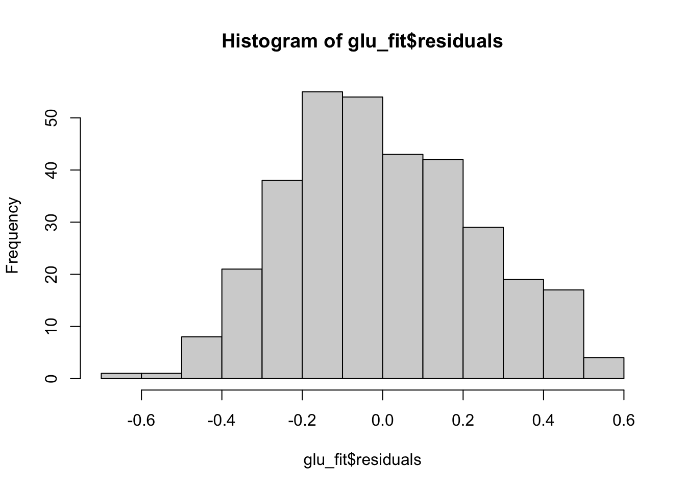
plot(x = glu_fit$fitted.values, y = glu_fit$residuals)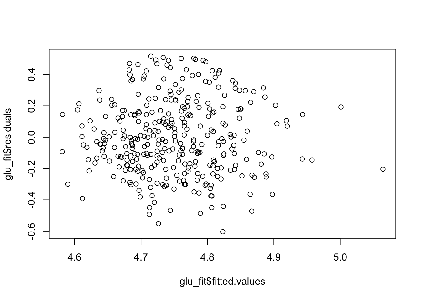
qqnorm(glu_fit$residuals)
qqline(glu_fit$residuals, col = "red")
Because these residual plots look quite good, we can then move on to interpreting the coefficients, doing hypothesis tests and constructing confidence intervals.
We also need to modify the definition of the residual standard error again, to account for the number of predictors in our model. The formula, which we saw before, is given by
\[ \hat{\sigma}_e = \sqrt{\frac{\sum_{i=1}^{n}(y_i - \hat{y}_i)^2}{n - p -1}}, \]
where we have \(p=3\) predictors here.
Interpreting the coefficients
How we interpret the coefficients is largely similar to what we did before, where we need to control for all other variables in our model. Looking at the output, we have \(\hat{\beta}_3=0.005\). This means that, under the fitted model, holding blood pressure and skin thickness fixed, a one unit increase in BMI leads to an average increase of the log glucose level of \(0.005\). Note that as was the case with only one predictor, we need to be a bit careful about the log transformation and the interpretation. These estimates only tell us about the relationship between \(\log Y\) and \(X\), not about \(Y\) and \(X\).
Testing the coefficients
We have seen that we can do two different types of tests for our coefficients:
An \(F\)-test, testing if all slope terms are zero
A regular \(t\)-test, for any one slope coefficient \(\beta_j\) while including all other predictors in the model
Recall that the \(F\)-test is used to test \(H_0:\beta_1=\beta_2 =\ldots =\beta_p =0\) vs \(H_A:\) at least one \(\beta_1,\beta_2,\ldots,\beta_p\neq 0\) at significance level \(\alpha\).
The test statistic \(f\) is
\[ f = \frac{MSModel}{MSError}, \]
which, under \(H_0\), follows an \(F\) distribution with \(p,n-p-1\) degrees of freedom. In this example we have \(p=3\) and the \(p\)-value, given by summary is less than \(\alpha =0.05\), so we would reject \(H_0\) at significance level \(\alpha\).
To test \(H_0:\beta_2=0\) vs \(H_A:\beta_2\neq 0\) at \(\alpha = 0.01\) for this example, we need the estimate, the standard error and the critical value of the corresponding \(t\)-distribution, which will have \(n-p-1\) degrees of freedom.
So in this example our test statistic will be
\[ t = \frac{0.0029-0}{0.00178} = 1.681 \]
and the critical value is \(t_{n-p-1=328, 0.005} = 2.59\), so because our test statistic is not further than 0 than the critical value, we fail to reject this \(H_0\).
Confidence and Prediction Intervals
We can also construct confidence and prediction intervals in this setting. These are very similar to what we saw before.
A \(100(1-\alpha)\%\) confidence interval for \(\beta_j\) will look like
\[ \left( \hat{\beta}_j - se(\hat{\beta}_j )t_{n-p-1,\alpha/2}, \hat{\beta}_j + se(\hat{\beta}_j )t_{n-p-1,\alpha/2} \right) \]
Note that if our model used \(\log(Y)\) instead of \(Y\), we cannot do a transformation to then say things about \(Y\) instead, using the confidence intervals for the coefficients.
We can also get confidence and prediction intervals for the response variable, \(Y\), even if we fit a model to some transformation of \(Y\). Again, these are quite similar to what we saw before, where again the standard errors will be too complex to show or calculate.
A \(100(1-\alpha)\%\) confidence interval for the average value of \(Y\), at values of the predictor variables \(x_1^{new},x_2^{new},\ldots,x_p^{new}\) will be
\[ \left( \hat{\beta}_0 +\hat{\beta}_1 x_1^{new}+\hat{\beta}_2 x_2^{new} + \ldots +\hat{\beta}_p x_p^{new}- t_{n-p-1,\alpha/2}S, \hat{\beta}_0 +\hat{\beta}_1 x_1^{new}+\hat{\beta}_2 x_2^{new} + \ldots + \hat{\beta}_p x_p^{new} + t_{n-p-1,\alpha/2}S \right). \]
Similarly, a \(100(1-\alpha)\%\) prediction interval will be
\[ \left( \hat{\beta}_0 +\hat{\beta}_1 x_1^{new}+\hat{\beta}_2 x_2^{new} + \ldots +\hat{\beta}_p x_p^{new}- t_{n-p-1,\alpha/2}S^*, \hat{\beta}_0 +\hat{\beta}_1 x_1^{new}+\hat{\beta}_2 x_2^{new} + \ldots + \hat{\beta}_p x_p^{new} + t_{n-p-1,\alpha/2}S^* \right), \]
where \(S^* > S\), as there is more uncertainty in predicting a new \(Y\) than the line at given values of \(x_1^{new},\ldots,x_p^{new}\).
For example, we can use the fitted model to predict the average log glucose level of someone with a bp of 80, a skin thickness measurement of 40 and a BMI of 25, or a prediction interval for a new person with those measurements.
new_data <- data.frame(bp = 80, skin = 40, bmi = 25)

predict(glu_fit, newdata = new_data, interval = c("confidence"),
        level = 0.95)
fit lwr upr
1 4.759401 4.679541 4.83926predict(glu_fit, newdata = new_data, interval = c("prediction"),
level = 0.95) fit lwr upr
1 4.759401 4.28649 5.232311For the intervals for \(Y\), we can transform these to get them on the original scale, by taking exp of the intervals.
exp(predict(glu_fit, newdata = new_data, interval = c("confidence"),
        level = 0.95))
fit lwr upr
1 116.676 107.7206 126.3758exp(predict(glu_fit, newdata = new_data, interval = c("prediction"),
level = 0.95)) fit lwr upr
1 116.676 72.71078 187.225Challenges
As we add more variables to a regression model we run into more things that can go wrong. One of the most common issues that occurs in regressions like this is when you have predictors in your model which are highly correlated. Lets see a quick example with \(p=3\) predictors.
library(palmerpenguins)

multi_fit <- lm(body_mass_g ~ bill_length_mm +
                  bill_depth_mm + flipper_length_mm,
                data = penguins)

summary(multi_fit)
Call:
lm(formula = body_mass_g ~ bill_length_mm + bill_depth_mm + flipper_length_mm,
    data = penguins)

Residuals:
     Min       1Q   Median       3Q      Max
-1054.94  -290.33   -21.91   239.04  1276.64

Coefficients:
                   Estimate Std. Error t value Pr(>|t|)
(Intercept)       -6424.765    561.469 -11.443   <2e-16 ***
bill_length_mm        4.162      5.329   0.781    0.435
bill_depth_mm        20.050     13.694   1.464    0.144
flipper_length_mm    50.269      2.477  20.293   <2e-16 ***
---
Signif. codes:  0 '***' 0.001 '**' 0.01 '*' 0.05 '.' 0.1 ' ' 1

Residual standard error: 393.4 on 338 degrees of freedom
  (2 observations deleted due to missingness)
Multiple R-squared:  0.7615,    Adjusted R-squared:  0.7594
F-statistic: 359.7 on 3 and 338 DF,  p-value: < 2.2e-16
Looking at this output, we get a large \(p\)-value for the coefficient related to bill_length, indicating it does not have a strong relationship with the weight of a penguin.
However, if we just run lm(body_mass_g ~ bill_length_mm, data = penguins), using only this predictor, this model says that the slope coefficient for bill_length_mm is statistically significant, and there is a strong linear relationship between them.
single_fit <- lm(body_mass_g ~ bill_length_mm, data = penguins)

summary(single_fit)
Call:
lm(formula = body_mass_g ~ bill_length_mm, data = penguins)

Residuals:
     Min       1Q   Median       3Q      Max
-1762.08  -446.98    32.59   462.31  1636.86

Coefficients:
               Estimate Std. Error t value Pr(>|t|)
(Intercept)     362.307    283.345   1.279    0.202
bill_length_mm   87.415      6.402  13.654   <2e-16 ***
---
Signif. codes:  0 '***' 0.001 '**' 0.01 '*' 0.05 '.' 0.1 ' ' 1

Residual standard error: 645.4 on 340 degrees of freedom
  (2 observations deleted due to missingness)
Multiple R-squared:  0.3542,    Adjusted R-squared:  0.3523
F-statistic: 186.4 on 1 and 340 DF,  p-value: < 2.2e-16
How come these two models give different results? What about if we also consider the model with just flipper_length_mm as the predictor?
fit_2 <- lm(body_mass_g ~ flipper_length_mm, data = penguins)

summary(fit_2)
Call:
lm(formula = body_mass_g ~ flipper_length_mm, data = penguins)

Residuals:
     Min       1Q   Median       3Q      Max
-1058.80  -259.27   -26.88   247.33  1288.69

Coefficients:
                   Estimate Std. Error t value Pr(>|t|)
(Intercept)       -5780.831    305.815  -18.90   <2e-16 ***
flipper_length_mm    49.686      1.518   32.72   <2e-16 ***
---
Signif. codes:  0 '***' 0.001 '**' 0.01 '*' 0.05 '.' 0.1 ' ' 1

Residual standard error: 394.3 on 340 degrees of freedom
  (2 observations deleted due to missingness)
Multiple R-squared:  0.759, Adjusted R-squared:  0.7583
F-statistic:  1071 on 1 and 340 DF,  p-value: < 2.2e-16
Compare the previous results to the estimated slope coefficient and standard error for the flipper length. The estimate changes from one model to the next, but the standard error is much larger when all variables are included compared to the model with only flipper length as an \(x\) variable. This is even more apparent when we look at the estimates for the slope of bill_length in the previous two models.
We can also look at the \(R^2\) for multi_fit and for fit_2. They are almost identical, but fit_2 only has 1 predictor while multi_fit has 3. What is happening here? This happens because we are running a regression with predictors which are highly correlated, which makes it challenging to disentangle the relationship between \(Y\) and any single \(X\) variable. This also leads to standard errors for all coefficients, \(\hat{\beta}\), increasing when we add more variables. In even more extreme examples, a model with one \(x\) variable can have an estimated slope which is positive, while adding more variables can cause the estimate of the same relationship to become negative!
This will be more obvious if we use ggpairs on this data, which identifies that some of these variables are highly correlated.
ggpairs(penguins[, c("body_mass_g", "flipper_length_mm",
                     "bill_length_mm", "bill_depth_mm")])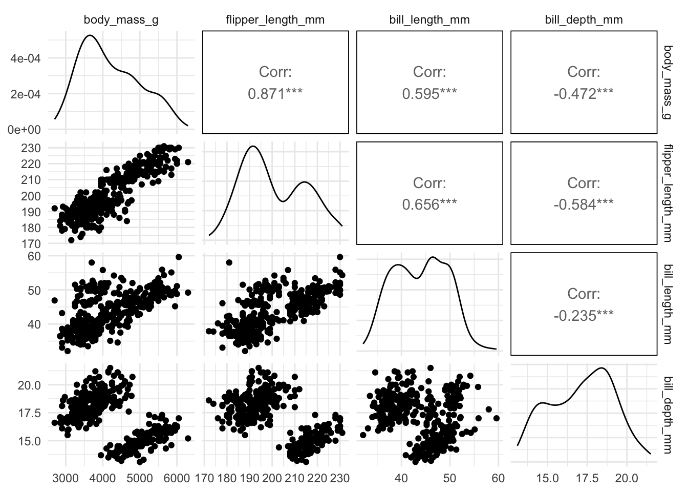
The other predictors all have quite large positive or negative correlation with flipper_length_mm, which leads to difficulties. Because these other predictors are highly correlated with flipper_length_mm, they aren’t able to give us much more information. This is why we see we don’t get a much improved model (in terms of \(R^2\)) by adding them to the model. This can also lead to problems with even getting estimates of the coefficients, and their standard errors, and so it may be incorrect to do hypothesis tests or construct intervals if you have very highly correlated variables.
Variance Inflation Factor
One thing we can do to identify problems like this, apart from using ggpairs to see which variables are highly correlated, is to compute something called the Variance Inflation Factor, which can help identify highly correlated variables.
The variance inflation factor for the \(j\)-th variable in the model is given by
\[ VIF_j = \frac{1}{1 - R_j^2}, \]
where \(R_j^2\) is the \(R^2\) value you get if you fit a regression where \(X_j\) is your \(Y\) variable and you use all other predictors in the model.
We can compute this using the vif function in the car package. Here we do it using a dataset of different car models, where we are interested in understanding the relationship between the price of a car and several other variables. Note that if we have categorical variables (later), an extension will be needed, which is why the output is called GVIF. This will give the same answers for all the examples we will consider.
library(MASS)
library(car)
## use this dataset from the MASS package
car_data <- Cars93

fit <- lm(Price ~ MPG.city + MPG.highway + Cylinders + EngineSize + Horsepower + Passengers,
          data = car_data)

summary(fit)
Call:
lm(formula = Price ~ MPG.city + MPG.highway + Cylinders + EngineSize +
    Horsepower + Passengers, data = car_data)

Residuals:
    Min      1Q  Median      3Q     Max
-15.509  -2.585  -0.754   1.721  31.993

Coefficients:
                Estimate Std. Error t value Pr(>|t|)
(Intercept)     17.10835   13.02500   1.314    0.193
MPG.city        -0.31589    0.44268  -0.714    0.478
MPG.highway     -0.04622    0.40308  -0.115    0.909
Cylinders4      -3.44972    4.63563  -0.744    0.459
Cylinders5       0.49253    6.91815   0.071    0.943
Cylinders6      -1.56899    5.74085  -0.273    0.785
Cylinders8       2.08057    7.17578   0.290    0.773
Cylindersrotary -8.01643    9.27716  -0.864    0.390
EngineSize      -1.59851    1.68297  -0.950    0.345
Horsepower       0.12696    0.02506   5.067 2.45e-06 ***
Passengers      -0.18214    0.88407  -0.206    0.837
---
Signif. codes:  0 '***' 0.001 '**' 0.01 '*' 0.05 '.' 0.1 ' ' 1

Residual standard error: 6.112 on 82 degrees of freedom
Multiple R-squared:  0.6431,    Adjusted R-squared:  0.5996
F-statistic: 14.78 on 10 and 82 DF, p-value: 1.209e-14vif(fit) GVIF Df GVIF^(1/(2*Df))
MPG.city 15.241506 1 3.904037
MPG.highway 11.374101 1 3.372551
Cylinders 14.399449 5 1.305673
EngineSize 7.506168 1 2.739739
Horsepower 4.240742 1 2.059306
Passengers 2.077728 1 1.441433We should be wary if we get large values of VIF
(the column called GVIF here) for any variables. One general heuristic is to try not have values of GVIF larger than 5, and definitely not larger than 10. For this example, if we remove some of the highly correlated variables, we will see these values decrease. This is probably not that surprising that when we have \(X\) variables for both the miles per gallon a car gets in a city and on the highway, they are highly correlated. We will also remove the number of cylinders.
cor(car_data$MPG.city, car_data$MPG.highway)[1] 0.9439358## removing mpg on highway and number of cylinders
fit <- lm(Price ~ MPG.city + EngineSize + Horsepower + Passengers,
data = car_data)
summary(fit)
Call:
lm(formula = Price ~ MPG.city + EngineSize + Horsepower + Passengers,
    data = car_data)

Residuals:
    Min      1Q  Median      3Q     Max
-15.250  -2.778  -1.142   1.860  32.060

Coefficients:
            Estimate Std. Error t value Pr(>|t|)
(Intercept)  4.95494    8.73593   0.567    0.572
MPG.city    -0.20349    0.18468  -1.102    0.274
EngineSize  -0.17242    1.07196  -0.161    0.873
Horsepower   0.13317    0.02192   6.075 3.08e-08 ***
Passengers   0.08108    0.79059   0.103    0.919
---
Signif. codes:  0 '***' 0.001 '**' 0.01 '*' 0.05 '.' 0.1 ' ' 1

Residual standard error: 6.016 on 88 degrees of freedom
Multiple R-squared:  0.629, Adjusted R-squared:  0.6121
F-statistic: 37.29 on 4 and 88 DF, p-value: < 2.2e-16vif(fit) MPG.city EngineSize Horsepower Passengers
2.738067 3.143335 3.350173 1.715094 Note that although we have removed 2 predictors, our \(R^2\) is almost the exact same value. Also, the standard errors look completely different. This is due to the high correlations that were present when we included the other predictors.
R-Squared
You might have noticed in the previous section that we often saw adding more predictor variables leads to only a small increase in the value of \(R^2\). It turns out, adding new predictors will always lead to an increase in \(R^2\), even if they are not appropriate. If we just add random data to our model, which is completely independent of \(Y\), it will still lead to a (small) increase in \(R^2\).
fit <- lm(Price ~ MPG.city + EngineSize + Horsepower + Passengers,
          data = car_data)

summary(fit)
Call:
lm(formula = Price ~ MPG.city + EngineSize + Horsepower + Passengers,
    data = car_data)

Residuals:
    Min      1Q  Median      3Q     Max
-15.250  -2.778  -1.142   1.860  32.060

Coefficients:
            Estimate Std. Error t value Pr(>|t|)
(Intercept)  4.95494    8.73593   0.567    0.572
MPG.city    -0.20349    0.18468  -1.102    0.274
EngineSize  -0.17242    1.07196  -0.161    0.873
Horsepower   0.13317    0.02192   6.075 3.08e-08 ***
Passengers   0.08108    0.79059   0.103    0.919
---
Signif. codes:  0 '***' 0.001 '**' 0.01 '*' 0.05 '.' 0.1 ' ' 1

Residual standard error: 6.016 on 88 degrees of freedom
Multiple R-squared:  0.629, Adjusted R-squared:  0.6121
F-statistic: 37.29 on 4 and 88 DF,  p-value: < 2.2e-16
## add random noise
noise <- rnorm(n = nrow(car_data))
car_data$noise <- noise
new_fit <- lm(Price ~ MPG.city + EngineSize + Horsepower + Passengers +
noise,
data = car_data)
summary(new_fit)
Call:
lm(formula = Price ~ MPG.city + EngineSize + Horsepower + Passengers +
    noise, data = car_data)

Residuals:
     Min       1Q   Median       3Q      Max
-15.6660  -2.9221  -0.9139   2.0742  30.8479

Coefficients:
            Estimate Std. Error t value Pr(>|t|)
(Intercept)  6.13886    8.74791   0.702    0.485
MPG.city    -0.21988    0.18436  -1.193    0.236
EngineSize  -0.11744    1.06849  -0.110    0.913
Horsepower   0.13287    0.02183   6.086 3.04e-08 ***
Passengers  -0.10399    0.80004  -0.130    0.897
noise        0.83579    0.63922   1.308    0.194
---
Signif. codes:  0 '***' 0.001 '**' 0.01 '*' 0.05 '.' 0.1 ' ' 1

Residual standard error: 5.992 on 87 degrees of freedom
Multiple R-squared:  0.6361,    Adjusted R-squared:  0.6152
F-statistic: 30.42 on 5 and 87 DF,  p-value: < 2.2e-16
Note that the computed \(R^2\) actually goes slightly up. When we have multiple \(X\) variables then \(R^2\) depends on the correlation between \(Y\) and \(\hat{Y}\), rather than between \(X\) and \(Y\). When we add a new variable, it can often lead to an increase in this correlation, even when the variable doesn’t have any true relationship with the \(Y\) variable of interest.
This is where the adjusted R squared, which is also given in the output of summary, finally comes into use. You’ll notice in this example, when we add the new \(x\) which is just random, the adjusted \(R^2\) actually decreases. This happened for the previous model with the additional variable also. It turns out that this other \(R^2\) can be used to give us information about whether to include a new predictor in our model.
Adjusted R-Squared
The adjusted R squared has a different definition to what we saw before.
Remember that
\[ R^2 = \frac{SSTotal - SSError}{SSTotal} = 1 - \frac{SSError}{SSTotal}. \]
This adjusted \(R^2\) accounts for the number of predictors \(p\) and the number of data points in our model, \(n\).
\[ R_{adj}^2 = 1-\frac{\frac{SSError}{n-p-1}}{\frac{SSTotal}{n-1}}. \]
If we remember the definition for \(\hat{\sigma}_{e}\), we can recognize that
\[ \hat{\sigma}_e^2 = \frac{SSError}{n-p-1} = \frac{\sum_{i}(y_i - \hat{y}_i)^2}{n-p-1}. \]
For the denominator, note that we previously said the sample variance of a sample given was by
\[ s_y^2 = \frac{1}{n}\sum_{i=1}^{n}(y_i -\bar{y})^2. \]
For technical (and most of the time not important) reasons 1, people often define this using \(n-1\) on the denominator,
\[ s_y^2 = \frac{1}{n-1}\sum_{i=1}^{n}(y_i -\bar{y})^2. \]
If we use this definition instead, then we can write this adjusted \(R^2\) as
\[ R_{adj}^2 = 1 - \frac{\hat{\sigma}_e^2}{s_y^2}. \] With this new definition of \(R_{adj}^2\), adding a new predictor which does not reduce the variability of the residuals by enough to account for the increase in \(p\) will lead to a smaller value of \(R_{adj}^2\).
3.5 Numeric and Binary Variables
The regression examples we have seen in this class so far has consisted of all variables being continuous. In practice, if you collect data you may have other types of variables, such as binary or categorical variables. For the penguin data, if we are interested in the weight of penguins, it probably makes sense to use the species of penguin in this model. We would like to include these variables in our regression model also. There are essentially two ways of doing this. We can:
Have a different intercept term for each group
Have a different slope term for each group
These two types of models will have different interpretations. Lets start with a simple example where we have a binary variable, the sex of penguins, which can be either male or female. We want to understand the relationship between their weight (\(Y\)) and their flipper length (\(X\)) while accounting for sex. We can see this with a plot, where we colour the points differently for male and female penguins.

We include sex as a predictor in our model, which we will call \(X_2\). \(X_1\) is the flipper length. Then, we can write a regression model as
\[ Y = \beta_0 + \beta_1 X_1 + \beta_2 X_2 + \epsilon. \]
When fitting this model in R, \(X_2\) can either be male or female. The way to handle this is to set \(X_2=0\) for one of these categories and \(X_2=1\) for the other. R does this alphabetically by default, so for a female penguin we will have \(X_2=0\) and for a male penguin \(X_2 = 1\). Lets think about how this model will change for the possible values of \(X_2\). When \(X_2=0\) then we will have
\[ Y =\beta_0 +\beta_1 X_1 +\epsilon\ \ \mathrm{(female)}, \]
while when \(X_2=1\) we will have
\[ Y = (\beta_0 + \beta_2) + \beta_1 X_1 +\epsilon \ \ \mathrm{(male)}. \]
We can call \(X_2\) an indicator variable, because its value indicates which group that observation is in. Essentially, we have a different intercept term for each group, but the same slope. This will result in two regression lines, one for each group, with the same slopes but different intercepts. This is shown in the next figure.

So we are basically fitting a separate line to each of the two groups, with the condition that they have to have the same slope.
Before we think about interpreting this model, we will see how to fit it and, like always, how to check the conditions for a regression model are satisfied.
bin_fit <- lm(body_mass_g ~ flipper_length_mm + sex,
              data = penguins)

summary(bin_fit)
Call:
lm(formula = body_mass_g ~ flipper_length_mm + sex, data = penguins)

Residuals:
    Min      1Q  Median      3Q     Max
-910.28 -243.89   -2.94  238.85 1067.73

Coefficients:
                   Estimate Std. Error t value Pr(>|t|)
(Intercept)       -5410.300    285.798 -18.931  < 2e-16 ***
flipper_length_mm    46.982      1.441  32.598  < 2e-16 ***
sexmale             347.850     40.342   8.623 2.78e-16 ***
---
Signif. codes:  0 '***' 0.001 '**' 0.01 '*' 0.05 '.' 0.1 ' ' 1

Residual standard error: 355.9 on 330 degrees of freedom
  (11 observations deleted due to missingness)
Multiple R-squared:  0.8058,    Adjusted R-squared:  0.8047
F-statistic: 684.8 on 2 and 330 DF,  p-value: < 2.2e-16
Checking the residuals is identical to before, because we are still just using lm.
hist(bin_fit$residuals)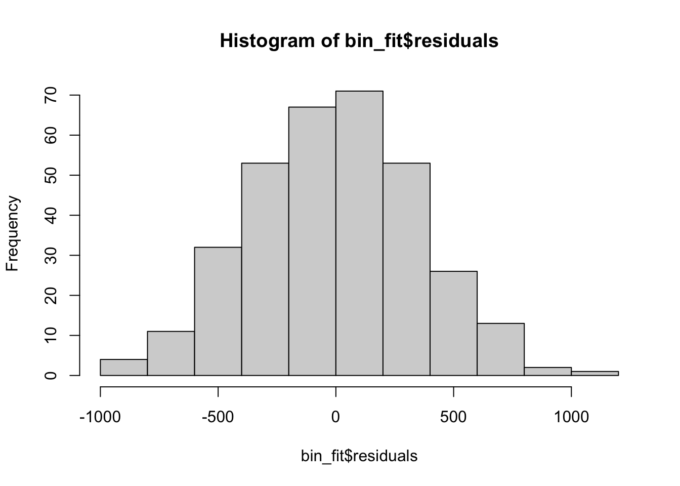
plot(x = bin_fit$fitted.values, y = bin_fit$residuals)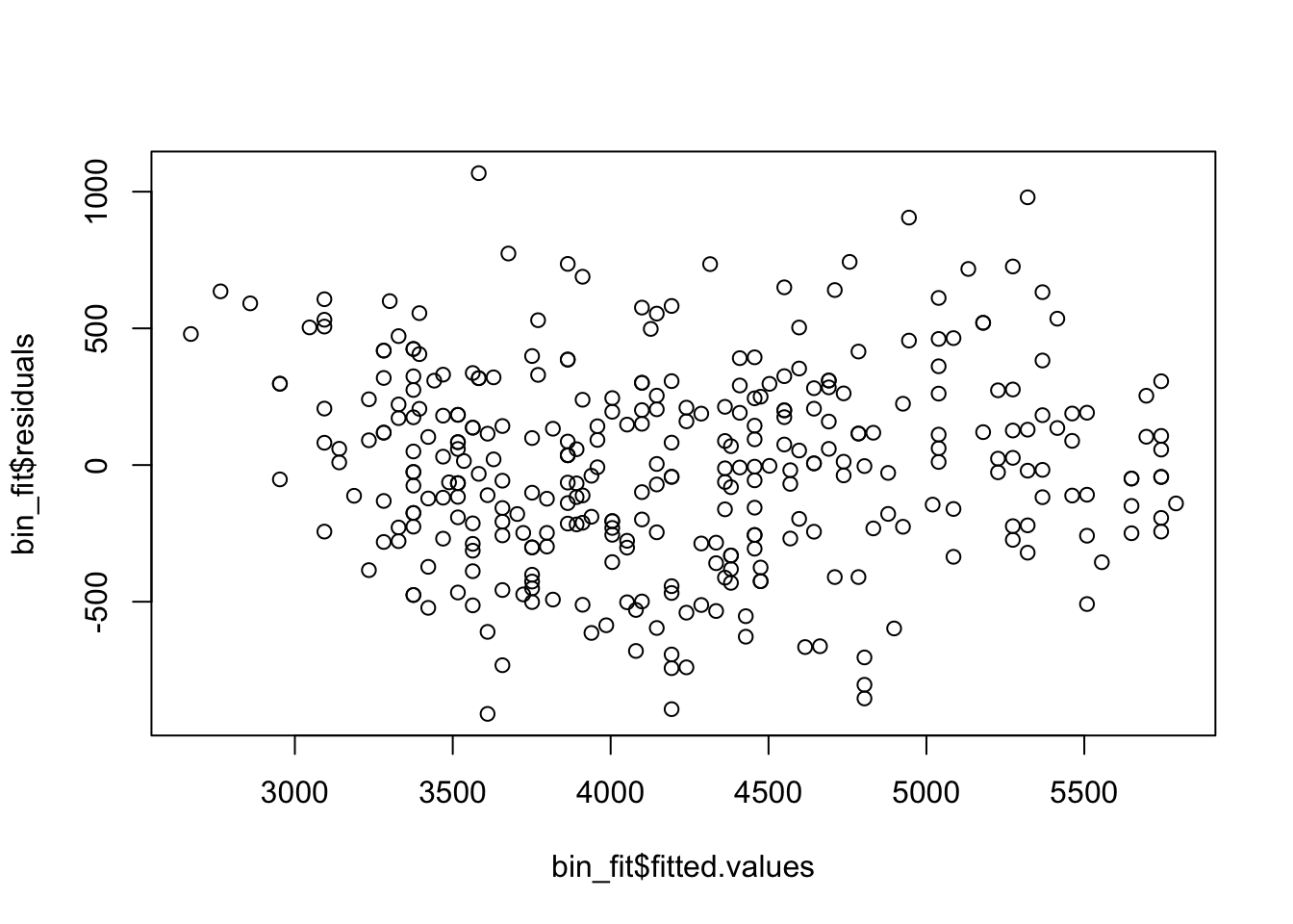
qqnorm(bin_fit$residuals)
qqline(bin_fit$residuals, col = "red")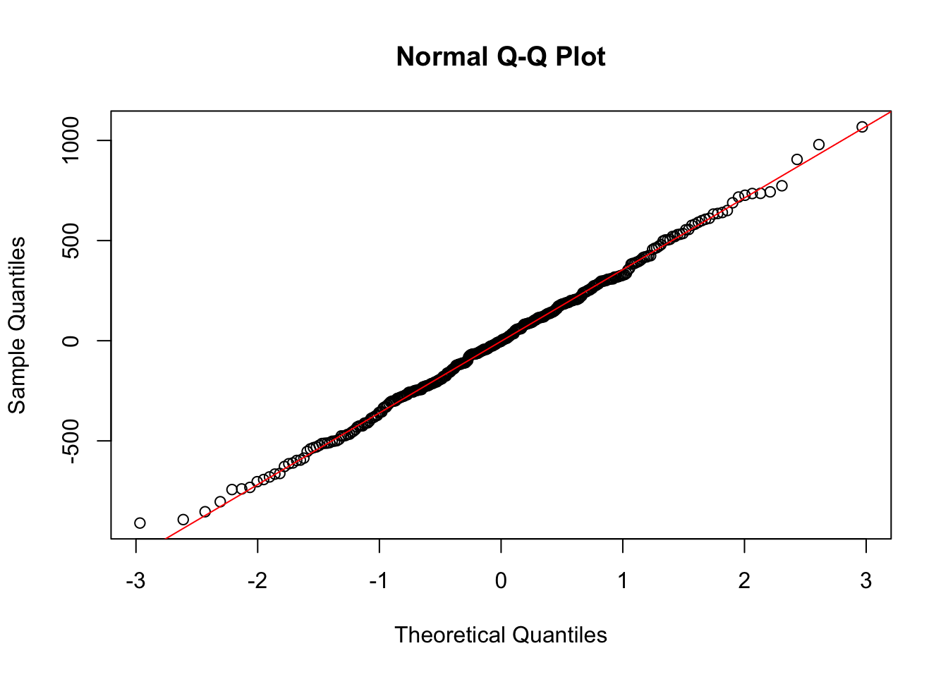
Here the residuals look very reasonable and we have no concerns about our regression model being valid. This means we can interpret the coefficients.
Now, the only thing which is different to what we saw before is how to interpret the intercept terms, \(\hat{\beta}_2\) and \(\hat{\beta}_0\). \(\hat{\beta}_0\) gives us the average weight for a female penguin with flipper length of 0. \(\hat{\beta}_2\) tells us about how the intercept changes from female to male penguins. What this says now is that if we have two penguins with the same flipper length, one male and one female, a male penguin will, on average, weigh \(\hat{\beta}_2\) grams more. Similarly, we can get a confidence interval for \(\beta_2\) using all the output we have above. This regression model allows us to describe the relationship between flipper length and body mass in the two groups of data at once.
We can also test \(H_0:\beta_2=0\) vs \(H_A:\beta_2\neq 0\) at \(\alpha=0.01\). We can get the critical value from a \(t\)-distribution with \(n-p-1\) degrees of freedom, where \(p=2\) here. Or, we can just look straight at the \(p\)-value in the output. Because this is smaller than \(\alpha\), we reject \(H_0\). Testing \(\beta_2\) means we are testing whether we need a different intercept for male and female penguins, or if we can describe the relationship between flipper length and body mass using just a single line for both male and female penguins.
Interactions
The previous model allowed us to have a different intercept for each of the two groups, which seemed to give a sensible model. However, what if we wanted to allow the slopes to vary across groups also?

To fit this model, we will write our regression in the following way, where we have the same variables as before,
\[ Y = \beta_0 +\beta_1 X_1 + \beta_2 X_2 + \beta_3 X_1 X_2 +\epsilon. \]
We call \(\beta_3 X_1 X_2\) an interaction term, describing the interaction between \(X_1\) and \(X_2\). Again, we will look at what happens when \(X_2=0\) and \(X_2=1\).
When \(X_2=0\) then we will have
\[ Y =\beta_0 +\beta_1 X_1 +\epsilon\ \ \mathrm{(female)}, \]
while when \(X_2=1\) we will have
\[ Y = (\beta_0 + \beta_2) + (\beta_1+\beta_3) X_1 +\epsilon \ \ \mathrm{(male)}. \]
So we will have a different slope and intercept for each of the two groups.
We can also fit this model using lm, where to include an interaction term we can write this as the product of the two \(x\) variables.
int_fit <- lm(body_mass_g ~ flipper_length_mm + sex + sex*flipper_length_mm,
              data = penguins)

summary(int_fit)
Call:
lm(formula = body_mass_g ~ flipper_length_mm + sex + sex * flipper_length_mm,
    data = penguins)

Residuals:
    Min      1Q  Median      3Q     Max
-909.36 -246.58   -3.13  237.18 1065.19

Coefficients:
                            Estimate Std. Error t value Pr(>|t|)
(Intercept)               -5443.9607   440.2829 -12.365   <2e-16 ***
flipper_length_mm            47.1527     2.2264  21.179   <2e-16 ***
sexmale                     406.8015   587.3029   0.693    0.489
flipper_length_mm:sexmale    -0.2942     2.9242  -0.101    0.920
---
Signif. codes:  0 '***' 0.001 '**' 0.01 '*' 0.05 '.' 0.1 ' ' 1

Residual standard error: 356.4 on 329 degrees of freedom
  (11 observations deleted due to missingness)
Multiple R-squared:  0.8058,    Adjusted R-squared:  0.8041
F-statistic: 455.2 on 3 and 329 DF,  p-value: < 2.2e-16
Again, we need to check the linear regression assumptions look to be satisfied before we can interpret this model and the estimates it gives.
hist(int_fit$residuals)
plot(x = int_fit$fitted.values, y = int_fit$residuals)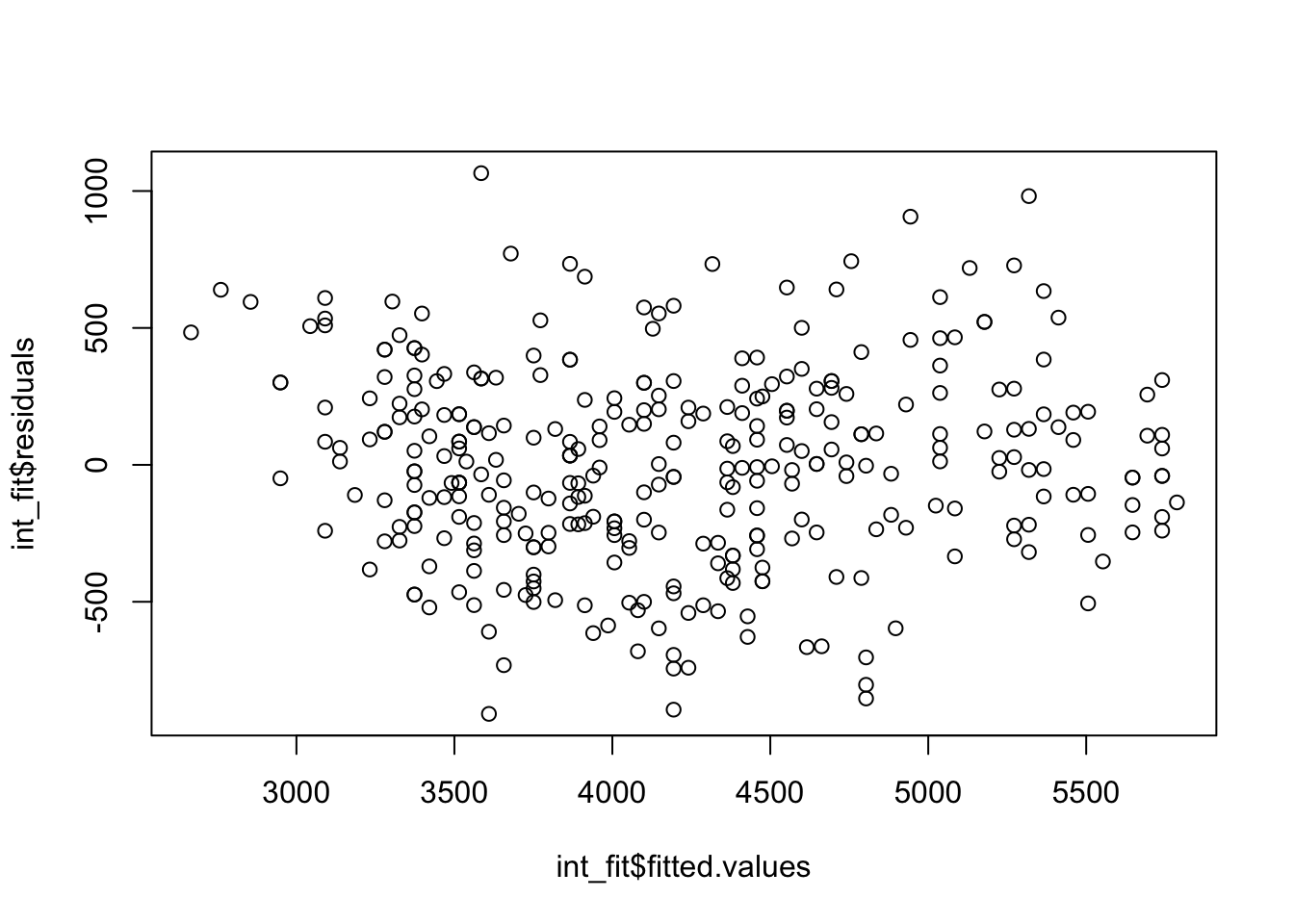
qqnorm(int_fit$residuals)
qqline(int_fit$residuals, col = "red")
Now we are saying there is an interaction between flipper length and sex, and the influence that flipper length has on the \(Y\) variable depends on the sex variable.
Comparing the slopes
Now an interesting question is whether we need a different slope for the two groups. From the plot, it seems like the slopes of these models are very similar, and we can examine this exactly by constructing confidence intervals or hypothesis tests for the value of \(\beta_3\), which is given by the last row of the summary output. Note that we have \(p=3\) slope coefficients \(\beta_1,\beta_2,\beta_3\), so the critical value will be from a t-distribution with \(n-p-1\) degrees of freedom.
For example, if we did a hypothesis test for \(H_0:\beta_3=0\) vs \(H_A:\beta_3\neq 0\) at \(\alpha=0.1\), we can see that the given \(p\)-value is 0.92, so we would fail to reject \(H_0\) at this significance level \(\alpha\). This means we have no evidence that there is a different slope for the two different groups.
We tested if \(\beta_2=0\) for the first model (different intercepts) and \(\beta_3=0\) for the second model (different slope and different intercept). We cannot do both these two tests for the same model to see if there is any relationship between the model and sex, because we would be doing multiple tests on the same data, which is a problem known as multiple testing. This means that the p-values given in summary are not correct if we use more than one of them. In a later section, we will see another method where we can use ANOVA techniques to investigate this.
3.6 Numeric and Categorical Variables
In the previous section we saw how to incorporate a binary variable into a regression model. What about a more general categorical variable, which can take more than 2 values? For the penguin data, the species variable is natural to include, and there are three species of penguin in this data. It makes sense to imagine that different species of penguins have different characteristics and incorporating them in a model would better describe this relationship.
It is slightly more complicated to include categorical variables in a regression model. Lets first consider a different slope for each of the 3 species. Lets first see the regression model in R and then we will describe the actual model that results in this code.
cat_fit <- lm(body_mass_g ~ flipper_length_mm + species,
              data = penguins)
summary(cat_fit)
Call:
lm(formula = body_mass_g ~ flipper_length_mm + species, data = penguins)

Residuals:
    Min      1Q  Median      3Q     Max
-927.70 -254.82  -23.92  241.16 1191.68

Coefficients:
                   Estimate Std. Error t value Pr(>|t|)
(Intercept)       -4031.477    584.151  -6.901 2.55e-11 ***
flipper_length_mm    40.705      3.071  13.255  < 2e-16 ***
speciesChinstrap   -206.510     57.731  -3.577 0.000398 ***
speciesGentoo       266.810     95.264   2.801 0.005392 **
---
Signif. codes:  0 '***' 0.001 '**' 0.01 '*' 0.05 '.' 0.1 ' ' 1

Residual standard error: 375.5 on 338 degrees of freedom
  (2 observations deleted due to missingness)
Multiple R-squared:  0.7826,    Adjusted R-squared:  0.7807
F-statistic: 405.7 on 3 and 338 DF,  p-value: < 2.2e-16
We have 3 species in this dataset but you’ll have noticed that we only get coefficients for two of the 3 species. This is because of the use of indicator variables.
We will create a variable \(X_2\) which is 1 if the penguin is Chinstrap, and 0 otherwise. Similarly, we will have \(X_3\), which is 1 is the penguin is Gentoo and 0 otherwise. So then the model is
\[ Y =\beta_0 + \beta_1 X_1 + \beta_2 X_2 + \beta_3 X_3 +\epsilon. \]
Lets consider what will happen for each of the three species. When the penguin is Adelie, then \(x_2=x_3=0\) and the model is
\[ Y = \beta_0 +\beta_1 x_1+\epsilon\ \ \textrm{(Adelie)}. \]
So for this group we will have intercept \(\beta_0\). When the penguin in Chinstrap then we have \(x_2=1\) and \(x_3=0\) giving
\[ Y = \beta_0 + \beta_2 +\beta_1 x_1+\epsilon\ \ \textrm{(Chinstrap)}. \]
For this group we will have intercept \(\beta_0 + \beta_2\). Finally, when we have a Gentoo penguin then \(x_2=0\) and \(x_3=1\) giving
\[ Y = \beta_0 +\beta_3 +\beta_1 x_1+\epsilon\ \ \textrm{(Gentoo)}. \]
For this group we will have intercept \(\beta_0 + \beta_3\). We will have the same slope \(\beta_1\) throughout. If our categorical variable has \(k\) categories then we need to include \(k-1\) variables to have all the categories in the model. We have a categorical variable for every category except the first, which is the baseline model. Then \(\beta_2\) and \(\beta_3\) tell us how much the other categories differ from that baseline. Again, this is done by default in alphabetical order.
We can see what the resulting model looks like, where we have the same slope but different intercepts for each species.
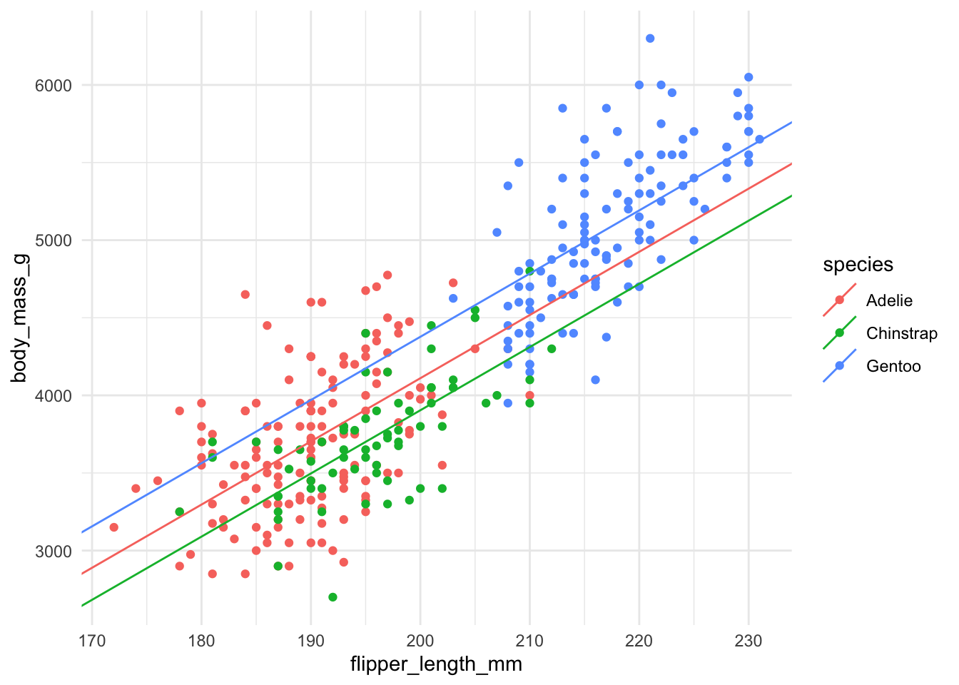
Once we check the residuals satisfy the required assumptions then we can again do hypothesis tests and confidence intervals and interpret these coefficients.
For example, \(\hat{\beta}_2\) now tells us how the intercept changes, on average, for Chinstrap penguins compared to Adelie penguins. All these interpretations are with respect to the first category, the baseline.
Just as before, we could also allow the intercept and the slope to vary for each of the categories. Again, this makes interpretation slightly more complicated, but all the ideas that we have seen now follow as before. The resulting regression lines are shown below.
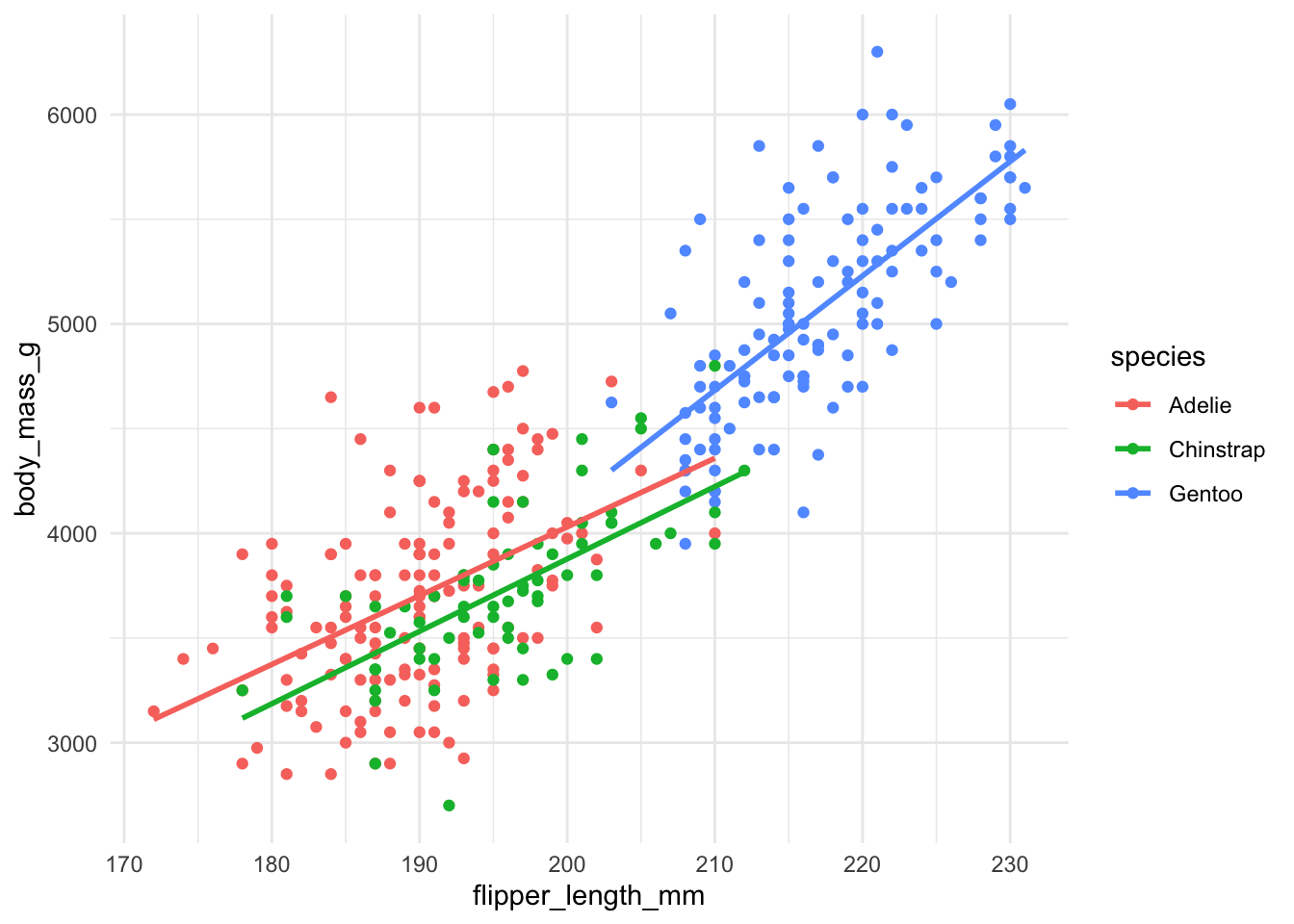
The regression formula for this model is then
\[ Y = \beta_0 + \beta_1 X_1 +\beta_2 X_2 +\beta_3 X_3 +\beta_4 X_1 X_2 + \beta_5 X_1 X_3 + \epsilon, \]
where we need an interaction between \(X_1\) and each of the categorical indicators. As before, we could consider testing whether we need a different intercept and/or slope for each of the groups, but these tests will require further ANOVA techniques which we will cover later in the semester. We will not discuss this model further, but by now you might be thinking that we could consider a lot of different models and its not clear how complicated we should go. The next section will provide some answers to these questions.
3.7 Model Complexity and Model Selection
We have now seen how we can go from a very simple regression model for \(Y\), with a single predictor \(X\), and extend this in numerous ways, incorporating many different types of variables and also functions of these variables. We now need to start thinking about how we actually decide on a model to use. Should we include \(X_1\) and \(X_2\) in our model? What about \(X_4\) or \(X_1^2\)?
While we only saw interactions previously between numeric and binary or categorical variables, we can actually have them between any types of variables we can put in our model. In theory, if you have 6 different predictors, you could have 15 potential interaction between any two of those variables! Very quickly, there are just too many different models to consider. Similarly, as we saw when looking at polynomial regression, it is easy to overfit a model to data if you include too many possible predictors.
We have seen already that we need a measure to quantify how “good” a model is, when we add additional variables, and that the regular \(R^2\) is no longer sufficient once we have more than one predictor. The adjusted R-squared improves over this, but we will see that there are other metrics we could consider also. We will see that we can actually use these methods to decide whether to include a variable as a predictor in our model or not. Or, if we have a model, we can use them to potentially remove an unnecessary predictor from our model.
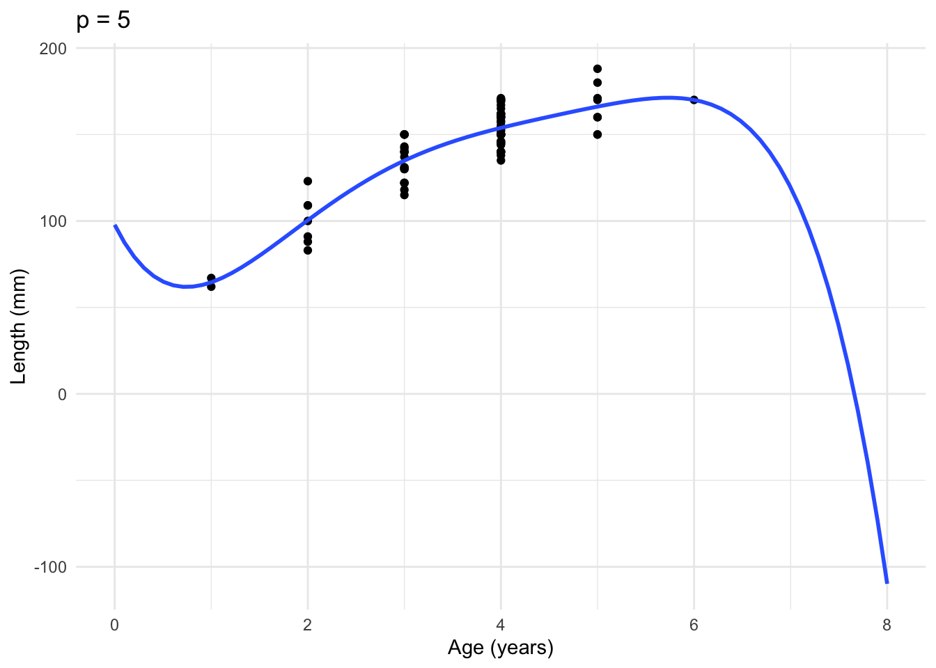
One way to see the problems of overfitting again is to look how a prediction interval can change as we make our model more complicated. Our prediction interval can actually get larger. This is most obvious when we try to predict at the edges of the observed data. We saw the fish data previously where we wanted to explore the relationship between the age of a fish (all 6 years or younger) and their length. We can compute a prediction interval for a 7 year old fish.
fit_quad <- lm(length ~ age + I(age^2), data = fish_data)

new_data <- data.frame(age = 7)

predict(fit_quad, new_data, interval = "prediction", level = 0.95)
fit lwr upr
1 160.753 127.664 193.8419## fit a polynomial of order 5, more flexible but possibly overfits
fit_comp <- lm(length ~ poly(age, 5), data = fish_data)
predict(fit_comp, new_data, interval = "prediction", level = 0.95) fit lwr upr
1 119.3607 -92.5985 331.32Here, we compare a quadratic model to a polynomial of order 5. The prediction interval for the \(p=5\) polynomial is useless. The estimated value is not even in the interval from the quadratic model. This is even more obvious when we plot the fitted regressions.
Similarly, while we quite easily interpret the relationships if we have one or two predictors in our model, as we add more predictors, and interactions between these predictors, it quickly becomes difficult to understand the model we are fitting. If we want to try use our regression to understand some scientific process, it would probably help if we can understand it. Then we might be able to explain what the coefficients mean, at least somewhat. Similarly, we probably don’t think all possible variables are actually “important”. It can be hard to interpret what variables are important when a model gets particularly complicated.
Example
Lets see an example of a particularly complicated model that is difficult to understand. Here we will use a dataset of house prices in Iowa. We have nearly 24 thousand houses and information for different 82 variables, which are numeric and categorical. We can include all these variables as predictors for the price of a house. This can be done in R using the notation lm(Y ~ .), where . indicates every other column in the data.
Because there are many categorical variables, this gives a model with \(p=270\) predictors! Looking at even just a small piece of this output, you would agree that it is difficult to interpret.
library(modeldata)
## the data is contained in this package

big_fit <- lm(Sale_Price ~ ., data = ames)
summ <- summary(big_fit)
summ$coefficients[1:20, ]
Estimate Std. Error
(Intercept) -2.083608e+07 10158540.656
MS_SubClassOne_Story_1945_and_Older 8.334772e+03 3272.755
MS_SubClassOne_Story_with_Finished_Attic_All_Ages 1.996254e+04 11128.340
MS_SubClassOne_and_Half_Story_Unfinished_All_Ages 1.283541e+04 13007.779
MS_SubClassOne_and_Half_Story_Finished_All_Ages 8.222432e+03 5996.520
MS_SubClassTwo_Story_1946_and_Newer -2.042516e+03 5174.432
MS_SubClassTwo_Story_1945_and_Older 1.345448e+04 5699.297
MS_SubClassTwo_and_Half_Story_All_Ages -4.881135e+03 9803.052
MS_SubClassSplit_or_Multilevel -9.261506e+03 10063.724
MS_SubClassSplit_Foyer -3.006487e+03 7029.075
MS_SubClassDuplex_All_Styles_and_Ages -2.169730e+04 5264.905
MS_SubClassOne_Story_PUD_1946_and_Newer -3.330004e+04 9650.056
MS_SubClassOne_and_Half_Story_PUD_All_Ages -3.584312e+04 27956.906
MS_SubClassTwo_Story_PUD_1946_and_Newer -3.653626e+04 11343.108
MS_SubClassPUD_Multilevel_Split_Level_Foyer -3.739830e+04 13291.602
MS_SubClassTwo_Family_conversion_All_Styles_and_Ages -7.677117e+03 16433.878
MS_ZoningResidential_High_Density 1.123161e+03 7011.875
MS_ZoningResidential_Low_Density 2.947611e+02 4686.779
MS_ZoningResidential_Medium_Density -3.503810e+03 5343.390
MS_ZoningA_agr -1.425126e+04 33705.666
t value Pr(>|t|)
(Intercept) -2.05108976 4.035600e-02
MS_SubClassOne_Story_1945_and_Older 2.54671395 1.093016e-02
MS_SubClassOne_Story_with_Finished_Attic_All_Ages 1.79384682 7.295120e-02
MS_SubClassOne_and_Half_Story_Unfinished_All_Ages 0.98674860 3.238557e-01
MS_SubClassOne_and_Half_Story_Finished_All_Ages 1.37120048 1.704282e-01
MS_SubClassTwo_Story_1946_and_Newer -0.39473247 6.930720e-01
MS_SubClassTwo_Story_1945_and_Older 2.36072582 1.831100e-02
MS_SubClassTwo_and_Half_Story_All_Ages -0.49791995 6.185816e-01
MS_SubClassSplit_or_Multilevel -0.92028620 3.575067e-01
MS_SubClassSplit_Foyer -0.42772154 6.688885e-01
MS_SubClassDuplex_All_Styles_and_Ages -4.12111836 3.885686e-05
MS_SubClassOne_Story_PUD_1946_and_Newer -3.45076120 5.677237e-04
MS_SubClassOne_and_Half_Story_PUD_All_Ages -1.28208457 1.999247e-01
MS_SubClassTwo_Story_PUD_1946_and_Newer -3.22100924 1.292808e-03
MS_SubClassPUD_Multilevel_Split_Level_Foyer -2.81367883 4.933814e-03
MS_SubClassTwo_Family_conversion_All_Styles_and_Ages -0.46715187 6.404295e-01
MS_ZoningResidential_High_Density 0.16017985 8.727516e-01
MS_ZoningResidential_Low_Density 0.06289203 9.498572e-01
MS_ZoningResidential_Medium_Density -0.65572785 5.120560e-01
MS_ZoningA_agr -0.42281505 6.724644e-01While many of these variables may have some relationship with the price of a house, we would like to identify the key variables, which have the biggest impact on the price of a house. We don’t want to claim that we will be able to find out the 4 or 5 variables that completely decide a price of a house, but we want to describe the data reasonably well with a model which we can interpret and potentially explain to others.
We will see several methods for selecting a subset of variables to use as our final regression model. We need a way to compare different models and so we will have several methods to determine a “good” model. These methods will compute different metrics and use them to decide whether to include a variable in the final model or not. One important point is to note how this differs from how we’ve done things previously. Before, we proposed a model and then fit that model. Once the regression residuals looked reasonable we could then interpret the model and do inference, such as tests and intervals for the coefficients. If we have not decided on our model in advance, inference for the coefficients is not valid. We cannot pick a model using the methods below and then test whether the coefficients are zero. We again run into problems related to multiple testing. We can interpret the coefficients, but only without statistical tests or confidence intervals.
Model Selection
We will now see some methods for choosing between models. There are many possible things you could do here, most of which are beyond the scope of this course. We will just highlight some possible tools.
We will consider:
All subsets regression
Backward Elimination
Forward Selection
Before we see these methods, we need to establish what metrics we will use to compare potential models.
Measures of Fit for Models
Previously we saw how \(R^2\) is not a reliable method for comparing models. To improve on this, we defined the adjusted \(R^2\), which accounts for the number of predictors in the model also. It will penalise models which add predictors which do not lead to a sufficient improvement in the variability of \(y\) described by the regression. Due to this penalty on the number of predictors in the model, if we compute \(R^2\) and \(R_{adj}^2\) for the same model, we will always have \(R_{adj}^2 < R^2\). We will now consider two more methods which have a similar goal to \(R_{adj}^2\).
The Akaike Information Criterion (AIC) accounts for the number of predictors in the model and prefers models which have smaller squared sums of errors. If we fit a model with \(p\) coefficients \(\beta_1,\beta_2,\ldots,\beta_p\) this model has sum of squares error \(SSError_{p}\), where we use \(p\) to denote a model with \(p\) coefficients. Then the AIC is defined as
\[ AIC = n\log(2\pi SSError_{p}/n) + n + 2p. \]
Note that this depends on \(n\), the number of observations in our dataset and also \(p\), the number of coefficients in our regression model. As we increase \(p\) the AIC will increase. As we increase \(n\), the first term may get smaller (as we divide by a larger number), while the second term, adding \(n\), will increase.
A very similar metric is known as the Bayesian Information Criterion (BIC) which is given by the formula
\[ BIC = n\log(2\pi SSError_{p}/n) + n + p\log n. \]
Note that the first two terms in AIC and BIC are identical, with the two formulas only differing on the last term. The first part, \(n\log(2\pi SSError_{p}/n)\) is something we try to minimise when fitting linear regression. It’s very similar and closely related to the least squares formula from Chapter 2. The final term is a penalty, and accounts for how complex the model is in terms of the number of coefficients \(p\) and/or the number of data points \(n\).
Unlike \(R_{adj}^2\), which we want to try get as close to 1 as possible, we want to minimize the AIC and the BIC. Increasing \(p\) will increase the AIC and BIC, and so unless increasing \(p\) leads to a sufficient reduction in \(n\log(2\pi SSError_{p}/n)\), we will have a higher AIC/BIC score, and a less desirable model.
\(R_{adj}^2\) is computed automatically when we run summary. For the AIC and BIC we need to run functions to compute these, AIC and BIC. Lets show these for some regression models we’ve seen before.
small_fit <- lm(body_mass_g ~ flipper_length_mm, data = penguins)
AIC(small_fit)
[1] 5062.855BIC(small_fit)[1] 5074.359big_fit <- lm(body_mass_g ~ flipper_length_mm + bill_length_mm +
bill_depth_mm, data = penguins)
AIC(big_fit)[1] 5063.32BIC(big_fit)[1] 5082.494If we use AIC or BIC to compare these two models, we see that the simpler model is preferred by both metrics.
We can also see the \(R_{adj}^2\) for these two models.
summary(small_fit)$adj.r.squared[1] 0.7582837summary(big_fit)$adj.r.squared[1] 0.7593534Note that the more complex model, with an additional predictor gives a slightly larger value of \(R_{adj}^2\). So if we only used \(R_{adj}^2\), we would prefer the more complicated model.
In general, if we use AIC or BIC or \(R_{adj}^2\) to compare models, they won’t necessarily give the same answer. Its easy to look at the scores from each of these metrics. If two models appear similar, its probably better to choose the simpler of the two models. This will be easier to explain and will do almost as well.
Now that we have a few different tools for comparing models, lets see how we can select models.
All Subsets Regression
We said that we might have more than \(p=100\) predictors when we include categorical variables, but we want to choose a simpler model which describes the data well. All subsets regression considers all possible subsets of these predictors and tries to pick the best model, from all these possibilities. We will show what this means using an example.
Example
Suppose we have collected data where we have \(3\) numeric predictor variables. The most general model, with all of these predictors, would be
\[ Y = \beta_0 + \beta_1 X_1 + \beta_2 X_2 +\beta_3 X_3 +\epsilon. \]
We have \(p=3\) predictors \(X_1,X_2,X_3\). All subsets means all possible subsets of these predictors in our model (excluding interactions). For each of the predictors, it can either be in the model or not. This means there are \(2^p=8\) possible models when \(p=3\). To make this extra clear, all the possibilities are
\[ Y = \beta_0 + \epsilon \\ \] \[ Y = \beta_0 + \beta_1 X_1 +\epsilon \\ \] \[ Y = \beta_0 + \beta_1 X_2 +\epsilon \\ \] \[ Y = \beta_0 + \beta_1 X_3 +\epsilon \\ \] \[ Y = \beta_0 + \beta_1 X_1 + \beta_2 X_2 + \epsilon \\ \] \[ Y = \beta_0 + \beta_1 X_1 + \beta_2 X_3 + \epsilon \\ \] \[ Y = \beta_0 + \beta_1 X_2 + \beta_2 X_3 + \epsilon \\ \] \[ Y = \beta_0 + \beta_1 X_1 + \beta_2 X_2 +\beta_3 X_3 + \epsilon. \\ \]
Here the interpretation of the slope terms will change between these models, depending on which variables are actually in the model. We are using \(\beta_1\) for the first predictor in the model, \(\beta_2\) for the second and so on. All subsets regression will consider all these models and pick the best one. Note that this is reasonable if \(p\) is not very large. However, if we have \(p=50\) possible numeric predictors, that is over a quadrillion possible models! We cannot fit and compare all these models in any reasonable amount of time. Lets see an example of doing this with the penguin data, which has \(p=7\) possible predictors. Some of these are categorical, meaning we will need even more coefficients to incorporate them in a regression.
Recall that we can consider a model with all possible predictors in a dataset by using the notation lm(y ~., data), where . allows the use of all possible predictors.
We will consider all such models here and then identify the 10 best models, that is the 10 models which give the smallest BIC score. The lmSelect function in the package lmSubsets allows us to fit all these possible models.
library(lmSubsets)

lm_bic <- lmSelect(body_mass_g ~ ., data = penguins,
                   penalty = "BIC", nbest = 10)

lm_bic
Call:
lmSelect(formula = body_mass_g ~ ., data = penguins, penalty = "BIC",
nbest = 10)
Criterion:
[best] = BIC
1st 2nd 3rd 4th 5th 6th 7th 8th
4752.472 4754.403 4755.232 4757.431 4758.279 4758.280 4759.567 4760.154
9th 10th
4760.231 4760.470
Subset:
best
+(Intercept) 1-10
speciesChinstrap 2-3,7-10
speciesGentoo 1-10
islandDream 4,8
islandTorgersen 5,7,10
bill_length_mm 2,6-9
bill_depth_mm 1-8,10
flipper_length_mm 1-10
sexmale 1-10 This gives quite a lot of different output, so we will explain the different components.
If we simply output lm_bic, this is an object which tells you about the best models and what variables they contain. The output tells you
The general linear regression model, under
call, similar to when we fit a single model.The
Criterion: gives us the BIC of the 10 best models, i.e the 10 smallest BIC scores, after fitting all \(2^p\) possible models.
Finally, the Subset: section goes through each of the possible predictors and identifies which of the 10 best models contain that predictor. For example, we see that all 10 of the best models contain Intercept,speciesGentoo,flipper_length_mm,sexmale, while islandDream is only included in the 4th and 8th best models.
Similarly, using the summary function on this gives some more useful output.
summary(lm_bic)Call:
lmSelect(formula = body_mass_g ~ ., data = penguins, penalty = "BIC",
nbest = 10)
Statistics:
SIZE BEST sigma R2 R2adj pval Cp AIC BIC
5 1 290.6573 0.8712718 0.8697020 < 2.22e-16 11.259976 4729.624 4752.472
7 2 287.3384 0.8749620 0.8726606 < 2.22e-16 5.678104 4723.938 4754.403
6 3 289.7720 0.8724449 0.8704945 < 2.22e-16 10.214035 4728.575 4755.232
6 4 290.7301 0.8716000 0.8696367 < 2.22e-16 12.407854 4730.774 4757.431
6 5 291.1007 0.8712725 0.8693041 < 2.22e-16 13.258404 4731.622 4758.279
6 6 291.1010 0.8712721 0.8693038 < 2.22e-16 13.259218 4731.623 4758.280
8 7 287.5016 0.8752038 0.8725159 < 2.22e-16 7.050099 4725.294 4759.567
8 8 287.7554 0.8749834 0.8722907 < 2.22e-16 7.622431 4725.881 4760.154
6 9 291.9553 0.8705155 0.8685356 < 2.22e-16 15.223959 4733.574 4760.231
7 10 289.9678 0.8726630 0.8703194 < 2.22e-16 11.647611 4730.005 4760.470Here for each of the 10 best models we get
Size: the number of predictors \(p\)Best: Where this specific model ranks in the best models in terms of BICsigma: An estimate of the residual standard errorR2: The \(R^2\) for that modelR2adj: The adjusted \(R^2\) for that modelpval: The p-Value for an \(F\)-test of \(H_0:\beta_1=\beta_2=\ldots=\beta_p=0\)Cp: Another metric we could use to compare models, which we don’t discuss in this class (and has a slightly different interpretation).AIC: The AIC for each of these models.BIC: The BIC for each of these models.
We can instead get the best models in terms of minimum AIC, by specifying penalty = "AIC" inside the function lmSelect. We can create all the exact same output. Note that when we do this we could get completely different models, and AIC picks a different model as the best model here.
lm_aic <- lmSelect(body_mass_g ~ ., data = penguins,
                   penalty = "AIC", nbest = 10)

lm_aic
Call:
lmSelect(formula = body_mass_g ~ ., data = penguins, penalty = "AIC",
nbest = 10)
Criterion:
[best] = AIC
1st 2nd 3rd 4th 5th 6th 7th 8th
4723.938 4725.294 4725.881 4727.242 4728.575 4729.624 4730.005 4730.570
9th 10th
4730.774 4731.622
Subset:
best
+(Intercept) 1-10
speciesChinstrap 1-5,7-8
speciesGentoo 1-10
islandDream 3-4,8-9
islandTorgersen 2,4,7,10
bill_length_mm 1-4
bill_depth_mm 1-10
flipper_length_mm 1-10
sexmale 1-10 summary(lm_aic)Call:
lmSelect(formula = body_mass_g ~ ., data = penguins, penalty = "AIC",
nbest = 10)
Statistics:
SIZE BEST sigma R2 R2adj pval Cp AIC BIC
7 1 287.3384 0.8749620 0.8726606 < 2.22e-16 5.678104 4723.938 4754.403
8 2 287.5016 0.8752038 0.8725159 < 2.22e-16 7.050099 4725.294 4759.567
8 3 287.7554 0.8749834 0.8722907 < 2.22e-16 7.622431 4725.881 4760.154
9 4 287.9227 0.8752231 0.8721422 < 2.22e-16 9.000000 4727.242 4765.324
6 5 289.7720 0.8724449 0.8704945 < 2.22e-16 10.214035 4728.575 4755.232
5 6 290.6573 0.8712718 0.8697020 < 2.22e-16 11.259976 4729.624 4752.472
7 7 289.9678 0.8726630 0.8703194 < 2.22e-16 11.647611 4730.005 4760.470
7 8 290.2136 0.8724471 0.8700995 < 2.22e-16 12.208383 4730.570 4761.035
6 9 290.7301 0.8716000 0.8696367 < 2.22e-16 12.407854 4730.774 4757.431
6 10 291.1007 0.8712725 0.8693041 < 2.22e-16 13.258404 4731.622 4758.279Note that these two metrics give different best models and can include some of the categories in a categorical predictor but not all. Recall that when we have a categorical predictor, with \(K\) categories, we need \(K-1\) indicator variables to encode it. These tools may pick some of these indicator variables but doesn’t have to include all of them.
Using AIC picks a different best model to when we use BIC. How should we decide between the two of them? In practice it may not make that much of a difference. One potential way to choose would be to pick the model with larger \(R_{adj}^2\). It’s also likely that using AIC or BIC will give models which differ only slightly. For this example here, the best model using BIC is
\[ Y = \beta_0 + \beta_1 flipperlength + \beta_2 sexmale + \beta_3 billdepth + \beta_4 speciesGentoo + \epsilon \]
while the best model using AIC is
\[ Y = \beta_0 + \beta_1 flipperlength + \beta_2 sexmale + \beta_3 billdepth + \beta_4 speciesGentoo + \beta_5 speciesChinstrap + \beta_6 billlength + \epsilon \]
which has 2 additional predictors. If you want to use these models for prediction (below), they will likely have quite similar performance.
Forward selection
All subsets Regression is only really useful when \(p\), the total number of predictors, is relatively small. We cannot use it once \(p\) is larger than 10.
An alternative method is then to consider starting with the simplest possible model, and attempt to iteratively add new predictors to it, until you reach some criterion to stop. This is how forward selection works.
We will fit this forward selection model and then explain the output. To fit this model, we cannot have any missing values in our datset, so we need to manually remove them, which we do using na.omit. Note that many other methods do this inside the function for you. It is important to be aware if you use a function which does this.
We specify a baseline model, i.e the simplest model. In general, and for this example, this will be a model with just an intercept, i.e
\[ Y = \beta_0 +\epsilon, \]
meaning there is no predictors in the model at all. We also specify the most complicated possible model, which here would include all 7 other variables we record. Then forward stepwise regression will “step” through these models. At each step, it will compute the AIC from adding one new predictor to the model, and compare this to keeping the previous version of the model instead (without that added predictor). It will stop stepping forward when adding a new predictor to the model does not give a better model (in terms of AIC).
The following output shows how this choice is made.
all_peng <- na.omit(penguins)

fullModel <- lm(body_mass_g ~ ., data = all_peng)
baseModel <- lm(body_mass_g ~ 1, data = all_peng)

forward_fit <- step(baseModel,
     scope = list(upper = fullModel, lower = ~1),
     direction="forward")
Start: AIC=4457.28
body_mass_g ~ 1
Df Sum of Sq RSS AIC
+ flipper_length_mm 1 164047703 51211963 3981.1
+ species 2 145190219 70069447 4087.5
+ island 2 83740680 131518986 4297.2
+ bill_length_mm 1 74792533 140467133 4317.1
+ bill_depth_mm 1 47959592 167300074 4375.3
+ sex 1 38878897 176380769 4392.9
<none> 215259666 4457.3
Step: AIC=3981.13
body_mass_g ~ flipper_length_mm
Df Sum of Sq RSS AIC
+ sex 1 9416589 41795374 3915.5
+ species 2 5368818 45843144 3948.3
+ island 2 3437527 47774435 3962.0
+ bill_depth_mm 1 338887 50873075 3980.9
<none> 51211963 3981.1
+ bill_length_mm 1 140000 51071963 3982.2
Step: AIC=3915.47
body_mass_g ~ flipper_length_mm + sex
Df Sum of Sq RSS AIC
+ species 2 13141806 28653568 3793.8
+ island 2 6037165 35758209 3867.5
+ bill_depth_mm 1 3667377 38127997 3886.9
<none> 41795374 3915.5
+ bill_length_mm 1 144990 41650383 3916.3
Step: AIC=3793.76
body_mass_g ~ flipper_length_mm + sex + species
Df Sum of Sq RSS AIC
+ bill_depth_mm 1 1196096 27457472 3781.6
+ bill_length_mm 1 780776 27872792 3786.6
<none> 28653568 3793.8
+ island 2 61695 28591873 3797.0
Step: AIC=3781.56
body_mass_g ~ flipper_length_mm + sex + species + bill_depth_mm
Df Sum of Sq RSS AIC
+ bill_length_mm 1 541825 26915647 3776.9
<none> 27457472 3781.6
+ island 2 59488 27397984 3784.8
Step: AIC=3776.93
body_mass_g ~ flipper_length_mm + sex + species + bill_depth_mm +
bill_length_mm
Df Sum of Sq RSS AIC
<none> 26915647 3776.9
+ island 2 56214 26859432 3780.2At each step, we consider all the predictors we could add to the model, fit a separate regression with each of those predictors added, and compute the AIC. If the AIC from adding no additional predictors is smaller than adding one, we stop and output that as the chosen model. We can then look at the final chosen model, and the estimates of the coefficients for this model.
forward_fit
Call:
lm(formula = body_mass_g ~ flipper_length_mm + sex + species +
    bill_depth_mm + bill_length_mm, data = all_peng)

Coefficients:
      (Intercept)  flipper_length_mm            sexmale   speciesChinstrap
         -1460.99              15.95             389.89            -251.48
    speciesGentoo      bill_depth_mm     bill_length_mm
          1014.63              67.22              18.20
By default, this uses AIC to choose the best model. If we want to instead use the BIC then we need to specify k = log(n) as an additional argument in the step function, where \(n\) is the number of data points, i.e the number of rows in our data. Note that it will still call this quantity AIC when it shows the output.
n <- nrow(all_peng)
step(baseModel,
     scope = list(upper = fullModel, lower = ~1),
     direction="forward", k = log(n))
Start: AIC=4461.09
body_mass_g ~ 1
Df Sum of Sq RSS AIC
+ flipper_length_mm 1 164047703 51211963 3988.7
+ species 2 145190219 70069447 4099.0
+ island 2 83740680 131518986 4308.6
+ bill_length_mm 1 74792533 140467133 4324.7
+ bill_depth_mm 1 47959592 167300074 4383.0
+ sex 1 38878897 176380769 4400.6
<none> 215259666 4461.1
Step: AIC=3988.75
body_mass_g ~ flipper_length_mm
Df Sum of Sq RSS AIC
+ sex 1 9416589 41795374 3926.9
+ species 2 5368818 45843144 3963.5
+ island 2 3437527 47774435 3977.2
<none> 51211963 3988.7
+ bill_depth_mm 1 338887 50873075 3992.3
+ bill_length_mm 1 140000 51071963 3993.6
Step: AIC=3926.9
body_mass_g ~ flipper_length_mm + sex
Df Sum of Sq RSS AIC
+ species 2 13141806 28653568 3812.8
+ island 2 6037165 35758209 3886.6
+ bill_depth_mm 1 3667377 38127997 3902.1
<none> 41795374 3926.9
+ bill_length_mm 1 144990 41650383 3931.5
Step: AIC=3812.8
body_mass_g ~ flipper_length_mm + sex + species
Df Sum of Sq RSS AIC
+ bill_depth_mm 1 1196096 27457472 3804.4
+ bill_length_mm 1 780776 27872792 3809.4
<none> 28653568 3812.8
+ island 2 61695 28591873 3823.7
Step: AIC=3804.41
body_mass_g ~ flipper_length_mm + sex + species + bill_depth_mm
Df Sum of Sq RSS AIC
+ bill_length_mm 1 541825 26915647 3803.6
<none> 27457472 3804.4
+ island 2 59488 27397984 3815.3
Step: AIC=3803.58
body_mass_g ~ flipper_length_mm + sex + species + bill_depth_mm +
bill_length_mm
Df Sum of Sq RSS AIC
<none> 26915647 3803.6
+ island 2 56214 26859432 3814.5
Call:
lm(formula = body_mass_g ~ flipper_length_mm + sex + species +
    bill_depth_mm + bill_length_mm, data = all_peng)

Coefficients:
      (Intercept)  flipper_length_mm            sexmale   speciesChinstrap
         -1460.99              15.95             389.89            -251.48
    speciesGentoo      bill_depth_mm     bill_length_mm
          1014.63              67.22              18.20
Another thing to note here is that at each step it orders the predictors to add to the model, based on which will lead to the smallest AIC. However, this order could change from one step to the next, as we add a new predictor to the model.
Backward Elimination
Note that when we did forward stepwise regression we had to specify direction = "forward" in our model. We can instead go backwards, starting from the most complicated model and removing predictors, until removing a predictor no longer leads to a better AIC.
Lets see this output and then we will walk through what it means, which is very similar to the forward model.
back_fit <- step(fullModel, direction = "backward")Start: AIC=3780.23
body_mass_g ~ species + island + bill_length_mm + bill_depth_mm +
flipper_length_mm + sex
Df Sum of Sq RSS AIC
- island 2 56214 26915647 3776.9
<none> 26859432 3780.2
- bill_length_mm 1 538552 27397984 3784.8
- bill_depth_mm 1 963531 27822963 3790.0
- flipper_length_mm 1 2529936 29389369 3808.2
- sex 1 5364097 32223530 3838.9
- species 2 7733709 34593142 3860.5
Step: AIC=3776.93
body_mass_g ~ species + bill_length_mm + bill_depth_mm + flipper_length_mm +
sex
Df Sum of Sq RSS AIC
<none> 26915647 3776.9
- bill_length_mm 1 541825 27457472 3781.6
- bill_depth_mm 1 957145 27872792 3786.6
- flipper_length_mm 1 2481143 29396790 3804.3
- sex 1 5482024 32397671 3836.7
- species 2 11183644 38099291 3888.6Here, because there are only 2 steps, its easier to explain the output. We first fit the model with all predictors and compute its AIC. Then we consider all the potential models where we remove one of the predictors, and compute the AIC for each. We see that the model without using island as a predictor has a smaller AIC, so our first step is to remove it from the model.
Then, after excluding island, we consider all possible models where we remove another predictor, and compute their AIC. None of these models have a smaller AIC than the model which doesn’t remove another predictor, so we stop here and choose this model as the best.
We can then see the chosen model and the estimated coefficients. In this example, both the forward and backward methods end up choosing the same model. But this will not happen in general!
back_fit
Call:
lm(formula = body_mass_g ~ species + bill_length_mm + bill_depth_mm +
    flipper_length_mm + sex, data = all_peng)

Coefficients:
      (Intercept)   speciesChinstrap      speciesGentoo     bill_length_mm
         -1460.99            -251.48            1014.63              18.20
    bill_depth_mm  flipper_length_mm            sexmale
            67.22              15.95             389.89
We can again use BIC to choose the model also. In this case, it gives the same result, but again, this doesn’t have to happen! Note again that it calls the term AIC although we are changing the definition by specifying k so that it actually corresponds to BIC (as we defined it).
## bic need to define n, specify k = log(n)
n <- nrow(all_peng)
step(fullModel, direction = "backward", k = log(n))
Start: AIC=3814.5
body_mass_g ~ species + island + bill_length_mm + bill_depth_mm +
flipper_length_mm + sex
Df Sum of Sq RSS AIC
- island 2 56214 26915647 3803.6
<none> 26859432 3814.5
- bill_length_mm 1 538552 27397984 3815.3
- bill_depth_mm 1 963531 27822963 3820.4
- flipper_length_mm 1 2529936 29389369 3838.7
- sex 1 5364097 32223530 3869.3
- species 2 7733709 34593142 3887.1
Step: AIC=3803.58
body_mass_g ~ species + bill_length_mm + bill_depth_mm + flipper_length_mm +
sex
Df Sum of Sq RSS AIC
<none> 26915647 3803.6
- bill_length_mm 1 541825 27457472 3804.4
- bill_depth_mm 1 957145 27872792 3809.4
- flipper_length_mm 1 2481143 29396790 3827.1
- sex 1 5482024 32397671 3859.5
- species 2 11183644 38099291 3907.7
Call:
lm(formula = body_mass_g ~ species + bill_length_mm + bill_depth_mm +
    flipper_length_mm + sex, data = all_peng)

Coefficients:
      (Intercept)   speciesChinstrap      speciesGentoo     bill_length_mm
         -1460.99            -251.48            1014.63              18.20
    bill_depth_mm  flipper_length_mm            sexmale
            67.22              15.95             389.89
This has been a very quick introduction to some potential methods for model selection with linear regression. We have three potential ways to identify a best model, all of which may choose a different model as being “best”. All subsets regression is not that useful if the number of predictors is large. In general, forward selection will pick a simpler model to backwards elimination. This is because it starts at the simplest model and only adds more predictors if they lead to an improvement. Backwards elimination starts with a complex model and only removes predictors if removing them leads to a better model.
Note that in these examples, we didn’t consider the possibility of interactions between the predictors. These methods can allow for that also, which leads to many more models to consider. However, in practice, it is common that interactions between predictors are unnecessary and make a model overly complicated. While they can help you get a better model, you should usually be cautious about including them.
There are also many other methods we could use, which we have not considered in this class. As we have seen already, different methods and different metrics can choose different models and there is no one best model. Given you choose a model, you should confirm a regression is reasonable by examining the coefficients and also the diagnostic residual plots, but you cannot make inferences about the coefficients (hypothesis tests or confidence intervals) following this model selection procedure.
In general, a smaller model is easier to explain. However, if we are interested in prediction, a more complicated model might be better. If you collected more data, you could then evaluate the model on this new data. We will see in the next section a brief introduction to this.
Model Selection for Prediction
The previous section considered identifying a “best” regression model. We used metrics such as the AIC and BIC to choose this best model, but we don’t have to. In some applications, you might be interested in the best regression model for prediction. That is, if you collect new data, which model would “best” predict the response variable, compared to the true values.
Like much of statistics, there are many ways we could define this best method for prediction. Here we will just see one method, and some quick examples of how to use it. Here overfitting can again be a problem, and we will see one way to avoid this in prediction.
How do we decide on whether a model is good at prediction, if we cannot easily collect new data? One way to do this is to split the data, into a training set and a test set. We will fit our model to the training data and then evaluate its performance on the test set. Splitting the data like this needs to be done carefully. All data should be as likely to be in the training set as the test set.
Lets do this with the penguin data. We will use approximately 75% of the data as the training data and 25% as the test data.
prob_train <- 0.75 ## probability any observation in the training data

all_penguins <- na.omit(penguins)

training_points <- sample(c(TRUE, FALSE), nrow(all_penguins), replace = TRUE,
                         prob = c(prob_train, 1-prob_train))


head(training_points)
[1] TRUE TRUE TRUE FALSE FALSE TRUEpenguin_train <- all_penguins[training_points, ]
penguin_test <- all_penguins[!training_points, ]This splits the data up into two groups. We first create a vector training_points, which has \(n\) elements, one for each row in the data set. If an entry in training_points is TRUE, then the same entry in the original data is in the training set. Otherwise, it is false and that entry is in the test set. Then penguins[training_points,] extracts the rows of the penguins data which are true, i.e, it just keeps the data in the training set.
Similarly, penguins[!training_points,] takes the points in the test set only. This is because ! flips the entries in training_points, turning TRUE to FALSE and vice versa. We can see this with the following example.
values <- c(TRUE, FALSE, TRUE, TRUE, FALSE)
!values
[1] FALSE TRUE FALSE FALSE TRUESo now we have our training set, penguin_train and our test set penguin_test. We can see how many of the total data points are in each, which is approximately 75% and 25%.
nrow(all_penguins)[1] 333nrow(penguin_train)[1] 256nrow(penguin_test)[1] 77nrow(penguin_train)/nrow(all_penguins)[1] 0.7687688Now we can fit a model on our training data to estimate the coefficients using that data. This will give us a model, and we will use that model to get predictions for the test data. We will compare those predictions to the true \(y\) values for the test data. We will use the model chosen by backward elimination with AIC here as an example.
train_model <- lm(body_mass_g ~ species + bill_length_mm + bill_depth_mm +
    flipper_length_mm + sex, data = penguin_train)

train_model
Call:
lm(formula = body_mass_g ~ species + bill_length_mm + bill_depth_mm +
    flipper_length_mm + sex, data = penguin_train)

Coefficients:
      (Intercept)   speciesChinstrap      speciesGentoo     bill_length_mm
         -1898.00            -293.22             982.62              18.78
    bill_depth_mm  flipper_length_mm            sexmale
            79.32              17.06             384.51
Note that because we are using the different data (the training data rather than all data), this will give us different estimates of the \(\beta\) coefficients than we saw above. But it is the same model, in that we are using the same variables as predictors.
We already know how to use this model to get predictions for the test data. This is very similar to getting prediction intervals, except now we are only interested in the fitted values \(\hat{y}\). We can do this using predict, and if we don’t specify a confidence level or a type of interval it will just give us the fitted values.
test_est <- predict(train_model, newdata = penguin_test)
head(test_est) ## look at the first few rows
1 2 3 4 5 6
3614.820 4100.073 3374.909 3346.694 3231.980 3748.710 How do we compare the predictions to the true values. There are many possible metrics but one we will consider here, which is quite commonly used, is mean squared error (MSE).
This is defined as
\[ MSE = \frac{1}{n_{test}}\sum_{i\in test}(y_i - \hat{y}_i)^2, \]
where \(n_{test}\) is the number of points in the test set. For each point in the test set, we compute \((y-\hat{y})^2\), The difference between the predicted value and the true value, squared. We then get the average of these.
## want to get mse of penguins_test$body_mass_g and test_est

mean((penguin_test$body_mass_g - test_est)^2)
[1] 93046.85This is just a number and so is maybe hard to interpret directly. However, we can compute this for alternative models and then compare them, assuming we use the same training and test data for both models.
We could also compute the correlation between the predicted values and the true values.
cor(penguin_test$body_mass_g, test_est)[1] 0.9254979We see that there is a high correlation, and this seems to indicate that our predictors are somewhat in agreement with the true values in the test set.
One important point to note is that we could also compute the MSE between the fitted values on the training data and the training data. That is, between the line estimated and the data used to estimate the line. This will normally lead to a smaller MSE and a higher correlation.
mean((train_model$fitted.values - penguin_train$body_mass_g)^2)[1] 77958.02cor(train_model$fitted.values, penguin_train$body_mass_g)[1] 0.9377801It is almost always the case that any model will perform better on the training data, because it is optimized for that data. This is related to overfitting, as we saw previously. However, the fact that the MSE and correlations are quite similar between the training and test results indicates this might be a good model.
We can compare this to a much simpler model, where we only use flipper_length as a predictor. Again, we fit this model with the training data and then evaluate these criteria on the test data.
simple_model <- lm(body_mass_g ~ flipper_length_mm, data = penguin_train)

simple_pred <- predict(simple_model, newdata = penguin_test)
mean((simple_pred - penguin_test$body_mass_g)^2)
[1] 147152cor(simple_pred, penguin_test$body_mass_g)[1] 0.8835852We see that this simpler model has much larger MSE and also smaller correlation, indicating it is not as good a predictive model.
If the main goal of a statistical model is prediction (which is not always the case), then a more complex model will often lead to better predictions. Evaluating the model on test data such as this can help prevent overfitting, where the model is excessively complex. There are many many other topics related to model selection for prediction, which we do not have time to cover further here, but are covered in other statistics courses!
3.8 Summary and Examples
There has been a large amount of material covered in this section, which has included
Fitting polynomial regressions
Fitting linear regressions with 2 or more explanatory (predictor) variables
The challenges which can occur with many explanatory (predictor) variables and how we can identify them
How to incorporate binary and categorical variables into a model
How we can choose between the many possible models we can consider for any specific problem.
We will finish this chapter by considering some worked examples where we use these methods for different data.
Example 1
Lets consider a dataset of prices of used cars. The first few rows of data are shown below.
library(modeldata)

head(car_prices)
# A tibble: 6 × 18
Price Mileage Cylinder Doors Cruise Sound Leather Buick Cadillac Chevy
<dbl> <int> <int> <int> <int> <int> <int> <int> <int> <int>
1 22661. 20105 6 4 1 0 0 1 0 0
2 21725. 13457 6 2 1 1 0 0 0 1
3 29143. 31655 4 2 1 1 1 0 0 0
4 30732. 22479 4 2 1 0 0 0 0 0
5 33359. 17590 4 2 1 1 1 0 0 0
6 30315. 23635 4 2 1 0 0 0 0 0
# ℹ 8 more variables: Pontiac <int>, Saab <int>, Saturn <int>,
# convertible <int>, coupe <int>, hatchback <int>, sedan <int>, wagon <int>We want to investigate the relationship between price and all other possible predictors. We will consider:
Checking to see if there is high correlation between these predictors
Choosing a possible model using forward stepwise regression
Note that here many of these predictors are binary. A car can either have leather seats or not, can be a Cadillac or not. The only numeric predictors are the milage, Cylinders and number of doors. Given that many of these predictors are binary, looking at the relationships using ggpairs will likely not be too useful. Because Price is positive and likely has a heavy tail (some very large values) we will do a log transformation of Price in fitting models.
We will first fit two possible models:
- A simple regression using just the mileage as a predictor for price
simple_fit <- lm(log(Price) ~ Mileage, data = car_prices)
summary(simple_fit)
Call:
lm(formula = log(Price) ~ Mileage, data = car_prices)

Residuals:
     Min       1Q   Median       3Q      Max
-0.77514 -0.32412 -0.09456  0.30831  1.17632

Coefficients:
              Estimate Std. Error t value Pr(>|t|)
(Intercept)  1.003e+01  3.749e-02 267.406  < 2e-16 ***
Mileage     -7.406e-06  1.747e-06  -4.239 2.51e-05 ***
---
Signif. codes:  0 '***' 0.001 '**' 0.01 '*' 0.05 '.' 0.1 ' ' 1

Residual standard error: 0.4058 on 802 degrees of freedom
Multiple R-squared:  0.02191,   Adjusted R-squared:  0.02069
F-statistic: 17.97 on 1 and 802 DF,  p-value: 2.511e-05
Note that if you examine the residuals for this simple model, a linear regression with just mileage does not appear to be an appropriate model for this data.
## Plots not shown, but regression assumptions not satisfied
hist(simple_fit$residuals)
qqnorm(simple_fit$residuals)
qqline(simple_fit$residuals)- Using all other variables as predictors for price
We can do this using ~., to specify we want all other variables in the dataset as predictors.
full_fit <- lm(log(Price) ~ ., data = car_prices)

summary(full_fit)
Call:
lm(formula = log(Price) ~ ., data = car_prices)

Residuals:
     Min       1Q   Median       3Q      Max
-0.30660 -0.07318  0.01288  0.07191  0.32388

Coefficients: (3 not defined because of singularities)
              Estimate Std. Error t value Pr(>|t|)
(Intercept)  8.770e+00  3.767e-02 232.835  < 2e-16 ***
Mileage     -8.209e-06  4.767e-07 -17.222  < 2e-16 ***
Cylinder     1.843e-01  4.301e-03  42.844  < 2e-16 ***
Doors        6.464e-02  9.825e-03   6.579 8.62e-11 ***
Cruise       2.860e-02  1.123e-02   2.546 0.011078 *
Sound        1.697e-02  8.898e-03   1.907 0.056824 .
Leather      3.611e-02  9.477e-03   3.810 0.000149 ***
Buick        8.822e-02  2.097e-02   4.207 2.88e-05 ***
Cadillac     4.006e-01  2.371e-02  16.896  < 2e-16 ***
Chevy       -3.073e-02  1.669e-02  -1.842 0.065856 .
Pontiac     -2.630e-02  1.847e-02  -1.424 0.154966
Saab         6.644e-01  2.105e-02  31.570  < 2e-16 ***
Saturn              NA         NA      NA       NA
convertible  2.807e-01  2.056e-02  13.649  < 2e-16 ***
coupe               NA         NA      NA       NA
hatchback   -2.889e-01  2.316e-02 -12.472  < 2e-16 ***
sedan       -1.765e-01  1.694e-02 -10.424  < 2e-16 ***
wagon               NA         NA      NA       NA
---
Signif. codes:  0 '***' 0.001 '**' 0.01 '*' 0.05 '.' 0.1 ' ' 1

Residual standard error: 0.1103 on 789 degrees of freedom
Multiple R-squared:  0.929, Adjusted R-squared:  0.9277
F-statistic: 736.9 on 14 and 789 DF,  p-value: < 2.2e-16
Looking at this fit we see that we get NA for several coefficients. This means that for some reason R is unable to estimate those values of \(\beta\). Why do you think that might be? For now, we will ignore this, and check the residuals for this regression model.
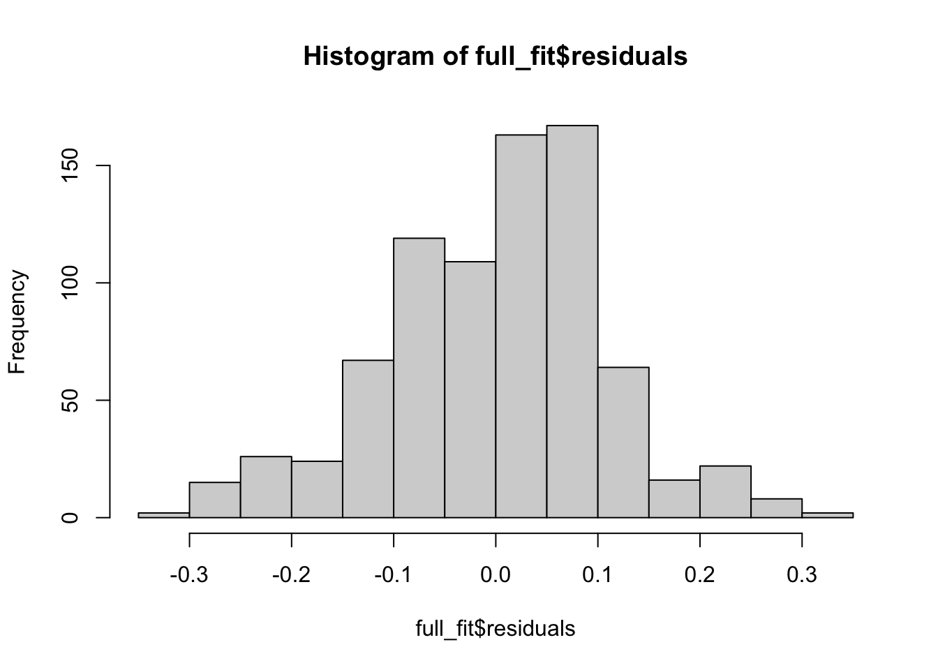

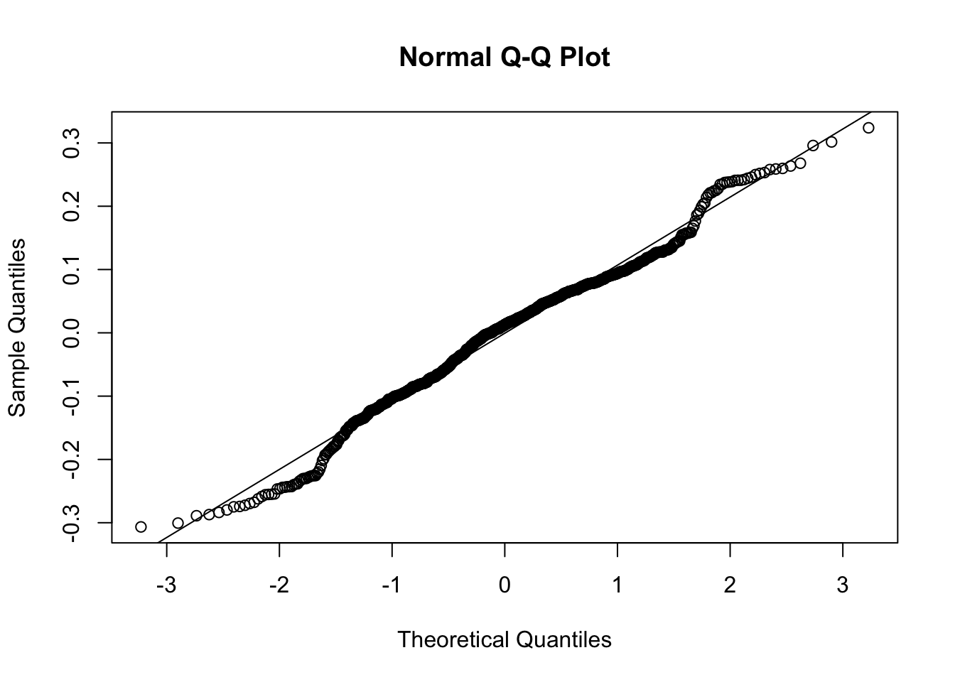
When we include all predictors we now see that the residuals look quite reasonable, and so a regression model might be appropriate now, when we include more predictors.
We saw that we have many predictors, and so we can investigate if these predictors are highly correlated. We will compute the vif scores for this.
library(car)
vif(full_fit)
Error in vif.default(full_fit): there are aliased coefficients in the modelWhen we try to compute the vif scores we get an error! This is related to the NA values we got above. It means that we have some exact dependence in our data, meaning some predictors are perfectly correlated. This is known as collinearity.
For example, if every coupe is also a Saturn, then these two variables are the exact same for all data and will be perfectly correlated.
We will remove the predictors which caused issues initially and see if we can remove these issues with correlated predictors.
largest_possible_fit <- lm(log(Price) ~ Mileage + Cylinder + Doors + Cruise +
                             Sound + Leather + Buick + Cadillac + Chevy +
                             Pontiac + Saab + convertible
                           + hatchback + sedan, data = car_prices)

summary(largest_possible_fit)
Call:
lm(formula = log(Price) ~ Mileage + Cylinder + Doors + Cruise +
    Sound + Leather + Buick + Cadillac + Chevy + Pontiac + Saab +
    convertible + hatchback + sedan, data = car_prices)

Residuals:
     Min       1Q   Median       3Q      Max
-0.30660 -0.07318  0.01288  0.07191  0.32388

Coefficients:
              Estimate Std. Error t value Pr(>|t|)
(Intercept)  8.770e+00  3.767e-02 232.835  < 2e-16 ***
Mileage     -8.209e-06  4.767e-07 -17.222  < 2e-16 ***
Cylinder     1.843e-01  4.301e-03  42.844  < 2e-16 ***
Doors        6.464e-02  9.825e-03   6.579 8.62e-11 ***
Cruise       2.860e-02  1.123e-02   2.546 0.011078 *
Sound        1.697e-02  8.898e-03   1.907 0.056824 .
Leather      3.611e-02  9.477e-03   3.810 0.000149 ***
Buick        8.822e-02  2.097e-02   4.207 2.88e-05 ***
Cadillac     4.006e-01  2.371e-02  16.896  < 2e-16 ***
Chevy       -3.073e-02  1.669e-02  -1.842 0.065856 .
Pontiac     -2.630e-02  1.847e-02  -1.424 0.154966
Saab         6.644e-01  2.105e-02  31.570  < 2e-16 ***
convertible  2.807e-01  2.056e-02  13.649  < 2e-16 ***
hatchback   -2.889e-01  2.316e-02 -12.472  < 2e-16 ***
sedan       -1.765e-01  1.694e-02 -10.424  < 2e-16 ***
---
Signif. codes:  0 '***' 0.001 '**' 0.01 '*' 0.05 '.' 0.1 ' ' 1

Residual standard error: 0.1103 on 789 degrees of freedom
Multiple R-squared:  0.929, Adjusted R-squared:  0.9277
F-statistic: 736.9 on 14 and 789 DF, p-value: < 2.2e-16vif(largest_possible_fit) Mileage Cylinder Doors Cruise Sound Leather
1.007864 2.351554 4.606826 1.553011 1.140603 1.186763
Buick Cadillac Chevy Pontiac Saab convertible
2.603970 3.329872 4.409925 3.424135 3.562993 1.630352
hatchback sedan
2.449436 4.513284 Now we get reasonable VIF values, indicating there may not be too many problems with these predictors. Note that we still get a large \(R_{adj}^2\).
Lets examine forward stepwise selection for this model to see how it differs from this current model, including all variables which are not exactly correlated.
fullModel <- lm(log(Price) ~ Mileage + Cylinder + Doors + Cruise + Sound +
                             Leather + Buick + Cadillac + Chevy + Pontiac + Saab + convertible
                           + hatchback + sedan, data = car_prices)
baseModel <- lm(log(Price) ~ 1, data = car_prices)

forward_fit <- step(baseModel,
     scope = list(upper = fullModel, lower = ~1),
     direction="forward")
Start: AIC=-1432.25
log(Price) ~ 1
Df Sum of Sq RSS AIC
+ Cylinder 1 45.947 89.110 -1764.6
+ Cadillac 1 45.442 89.616 -1760.0
+ Cruise 1 32.909 102.149 -1654.8
+ Chevy 1 29.393 105.665 -1627.6
+ convertible 1 26.181 108.877 -1603.5
+ Saab 1 21.875 113.182 -1572.3
+ hatchback 1 7.979 127.078 -1479.2
+ Mileage 1 2.959 132.099 -1448.1
+ Sound 1 2.619 132.439 -1446.0
+ Leather 1 2.285 132.773 -1444.0
+ Pontiac 1 1.195 133.862 -1437.4
+ Doors 1 1.133 133.925 -1437.0
<none> 135.058 -1432.2
+ Buick 1 0.264 134.793 -1431.8
+ sedan 1 0.006 135.051 -1430.3
Step: AIC=-1764.58
log(Price) ~ Cylinder
Df Sum of Sq RSS AIC
+ Saab 1 60.124 28.986 -2665.5
+ convertible 1 22.170 66.940 -1992.6
+ Chevy 1 19.437 69.674 -1960.4
+ Cadillac 1 13.595 75.516 -1895.7
+ Cruise 1 12.720 76.391 -1886.4
+ hatchback 1 6.030 83.081 -1818.9
+ Pontiac 1 3.540 85.571 -1795.2
+ Mileage 1 2.314 86.797 -1783.7
+ sedan 1 1.358 87.753 -1774.9
+ Doors 1 1.165 87.946 -1773.2
+ Sound 1 1.029 88.082 -1771.9
+ Leather 1 1.005 88.105 -1771.7
+ Buick 1 0.469 88.641 -1766.8
<none> 89.110 -1764.6
Step: AIC=-2665.51
log(Price) ~ Cylinder + Saab
Df Sum of Sq RSS AIC
+ Cadillac 1 9.4036 19.583 -2978.8
+ Mileage 1 3.6152 25.371 -2770.6
+ convertible 1 3.3528 25.634 -2762.3
+ hatchback 1 1.7773 27.209 -2714.4
+ Chevy 1 1.5233 27.463 -2706.9
+ Doors 1 0.7602 28.226 -2684.9
+ Leather 1 0.5413 28.445 -2678.7
+ Pontiac 1 0.3731 28.613 -2673.9
+ sedan 1 0.2801 28.706 -2671.3
+ Cruise 1 0.1147 28.872 -2666.7
<none> 28.986 -2665.5
+ Buick 1 0.0084 28.978 -2663.7
+ Sound 1 0.0000 28.986 -2663.5
Step: AIC=-2978.81
log(Price) ~ Cylinder + Saab + Cadillac
Df Sum of Sq RSS AIC
+ Mileage 1 3.2789 16.304 -3124.1
+ convertible 1 2.9788 16.604 -3109.5
+ Doors 1 1.4355 18.147 -3038.0
+ hatchback 1 1.2841 18.299 -3031.3
+ sedan 1 0.7532 18.830 -3008.3
+ Buick 1 0.4439 19.139 -2995.2
+ Chevy 1 0.3689 19.214 -2992.1
+ Cruise 1 0.2025 19.380 -2985.2
<none> 19.583 -2978.8
+ Pontiac 1 0.0296 19.553 -2978.0
+ Leather 1 0.0209 19.562 -2977.7
+ Sound 1 0.0159 19.567 -2977.5
Step: AIC=-3124.14
log(Price) ~ Cylinder + Saab + Cadillac + Mileage
Df Sum of Sq RSS AIC
+ convertible 1 3.05638 13.248 -3289.0
+ Doors 1 1.49077 14.813 -3199.2
+ hatchback 1 1.37876 14.925 -3193.2
+ sedan 1 0.76443 15.540 -3160.7
+ Buick 1 0.51270 15.791 -3147.8
+ Chevy 1 0.38748 15.917 -3141.5
+ Cruise 1 0.23334 16.071 -3133.7
<none> 16.304 -3124.1
+ Leather 1 0.02500 16.279 -3123.4
+ Pontiac 1 0.01500 16.289 -3122.9
+ Sound 1 0.00683 16.297 -3122.5
Step: AIC=-3289.04
log(Price) ~ Cylinder + Saab + Cadillac + Mileage + convertible
Df Sum of Sq RSS AIC
+ hatchback 1 1.33186 11.916 -3372.2
+ Buick 1 0.70159 12.546 -3330.8
+ Chevy 1 0.62141 12.626 -3325.7
+ Cruise 1 0.29401 12.954 -3305.1
+ Doors 1 0.16156 13.086 -3296.9
+ sedan 1 0.08813 13.159 -3292.4
+ Pontiac 1 0.05779 13.190 -3290.6
+ Leather 1 0.03506 13.213 -3289.2
<none> 13.248 -3289.0
+ Sound 1 0.00309 13.245 -3287.2
Step: AIC=-3372.23
log(Price) ~ Cylinder + Saab + Cadillac + Mileage + convertible +
hatchback
Df Sum of Sq RSS AIC
+ sedan 1 0.66252 11.253 -3416.2
+ Buick 1 0.49749 11.418 -3404.5
+ Chevy 1 0.20294 11.713 -3384.0
+ Leather 1 0.10511 11.811 -3377.4
+ Cruise 1 0.08258 11.833 -3375.8
+ Doors 1 0.03779 11.878 -3372.8
<none> 11.916 -3372.2
+ Sound 1 0.01232 11.903 -3371.1
+ Pontiac 1 0.00083 11.915 -3370.3
Step: AIC=-3416.23
log(Price) ~ Cylinder + Saab + Cadillac + Mileage + convertible +
hatchback + sedan
Df Sum of Sq RSS AIC
+ Buick 1 0.86221 10.391 -3478.3
+ Doors 1 0.59226 10.661 -3457.7
+ Chevy 1 0.25222 11.001 -3432.5
+ Cruise 1 0.09532 11.158 -3421.1
+ Leather 1 0.05269 11.201 -3418.0
<none> 11.253 -3416.2
+ Sound 1 0.01631 11.237 -3415.4
+ Pontiac 1 0.00579 11.248 -3414.6
Step: AIC=-3478.32
log(Price) ~ Cylinder + Saab + Cadillac + Mileage + convertible +
hatchback + sedan + Buick
Df Sum of Sq RSS AIC
+ Doors 1 0.48246 9.9086 -3514.5
+ Leather 1 0.14584 10.2452 -3487.7
+ Pontiac 1 0.04159 10.3495 -3479.5
+ Chevy 1 0.03313 10.3580 -3478.9
+ Cruise 1 0.02590 10.3652 -3478.3
<none> 10.3911 -3478.3
+ Sound 1 0.02001 10.3711 -3477.9
Step: AIC=-3514.54
log(Price) ~ Cylinder + Saab + Cadillac + Mileage + convertible +
hatchback + sedan + Buick + Doors
Df Sum of Sq RSS AIC
+ Leather 1 0.172516 9.7361 -3526.7
+ Sound 1 0.062009 9.8466 -3517.6
+ Cruise 1 0.051747 9.8569 -3516.7
<none> 9.9086 -3514.5
+ Pontiac 1 0.001063 9.9076 -3512.6
+ Chevy 1 0.000299 9.9083 -3512.6
Step: AIC=-3526.66
log(Price) ~ Cylinder + Saab + Cadillac + Mileage + convertible +
hatchback + sedan + Buick + Doors + Leather
Df Sum of Sq RSS AIC
+ Cruise 1 0.069140 9.6670 -3530.4
+ Sound 1 0.030417 9.7057 -3527.2
<none> 9.7361 -3526.7
+ Chevy 1 0.008827 9.7273 -3525.4
+ Pontiac 1 0.000008 9.7361 -3524.7
Step: AIC=-3530.39
log(Price) ~ Cylinder + Saab + Cadillac + Mileage + convertible +
hatchback + sedan + Buick + Doors + Leather + Cruise
Df Sum of Sq RSS AIC
+ Sound 1 0.0301676 9.6368 -3530.9
<none> 9.6670 -3530.4
+ Chevy 1 0.0098503 9.6571 -3529.2
+ Pontiac 1 0.0001541 9.6668 -3528.4
Step: AIC=-3530.9
log(Price) ~ Cylinder + Saab + Cadillac + Mileage + convertible +
hatchback + sedan + Buick + Doors + Leather + Cruise + Sound
Df Sum of Sq RSS AIC
<none> 9.6368 -3530.9
+ Chevy 1 0.0166459 9.6202 -3530.3
+ Pontiac 1 0.0000298 9.6368 -3528.9Using forward stepwise regression with AIC we get a model which retains all of these variables, except for Chevy and Pontiac. This is not that surprising as we saw that the regression with all these predictors had a high \(R_{adj}^2\). So using AIC we also keep most of these variables in our model.
Example 2
In this example we will consider a regression where we have both a binary and a categorical variable and we would like to include both of these in the model. We will look at data recorded for caterpillars, where we want to understand the relationship between their mass and some other variables we record. Our \(Y\) variable will be LogMass. We will have several predictors:
Instar, which gives the stage of life of the caterpillar, from 1 to 5. We will make this a categorical variableLogIntake, the log of the amount eaten by the caterpillarActiveFeeding, a binary variable indicating whether the caterpillar is in an active feeding state or not.
Note that Instar is coded taking values from 1 to 5, where 1 is the first stage and 5 is the last stage. As this is coded numerically, if we just fit a regression directly, R will treat it as a numeric variable. This may be ok but you would need some scientific knowledge to be certain. We don’t know anything here, so we will force R to treat this as a categorical variable. The function as.factor() will make it categorical, where all possible values (here 1-5) are the possible categories.
library(Stat2Data) ## to load the package with the data

data("Caterpillars") ## to load the data


fit <- lm(LogMass ~ LogIntake + as.factor(Instar) + ActiveFeeding,
          data = Caterpillars)

summary(fit)
Call:
lm(formula = LogMass ~ LogIntake + as.factor(Instar) + ActiveFeeding,
    data = Caterpillars)

Residuals:
     Min       1Q   Median       3Q      Max
-0.71593 -0.16988  0.03482  0.16247  0.61452

Coefficients:
                   Estimate Std. Error t value Pr(>|t|)
(Intercept)        -1.59967    0.09791 -16.339  < 2e-16 ***
LogIntake           0.80508    0.09779   8.233 8.92e-15 ***
as.factor(Instar)2  0.61805    0.05390  11.467  < 2e-16 ***
as.factor(Instar)3  1.15078    0.06109  18.837  < 2e-16 ***
as.factor(Instar)4  1.74701    0.08671  20.147  < 2e-16 ***
as.factor(Instar)5  2.11834    0.14683  14.427  < 2e-16 ***
ActiveFeedingY     -0.41256    0.03700 -11.149  < 2e-16 ***
---
Signif. codes:  0 '***' 0.001 '**' 0.01 '*' 0.05 '.' 0.1 ' ' 1

Residual standard error: 0.2423 on 260 degrees of freedom
Multiple R-squared:  0.9615,    Adjusted R-squared:  0.9606
F-statistic:  1082 on 6 and 260 DF,  p-value: < 2.2e-16
We can examine the residuals of this model to check it is reasonable, with these plots shown below.
hist(fit$residuals)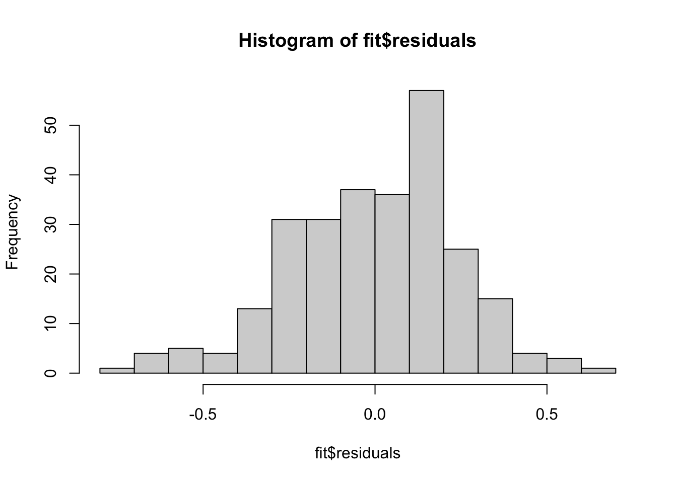
plot(x = fit$fitted.values, y = fit$residuals)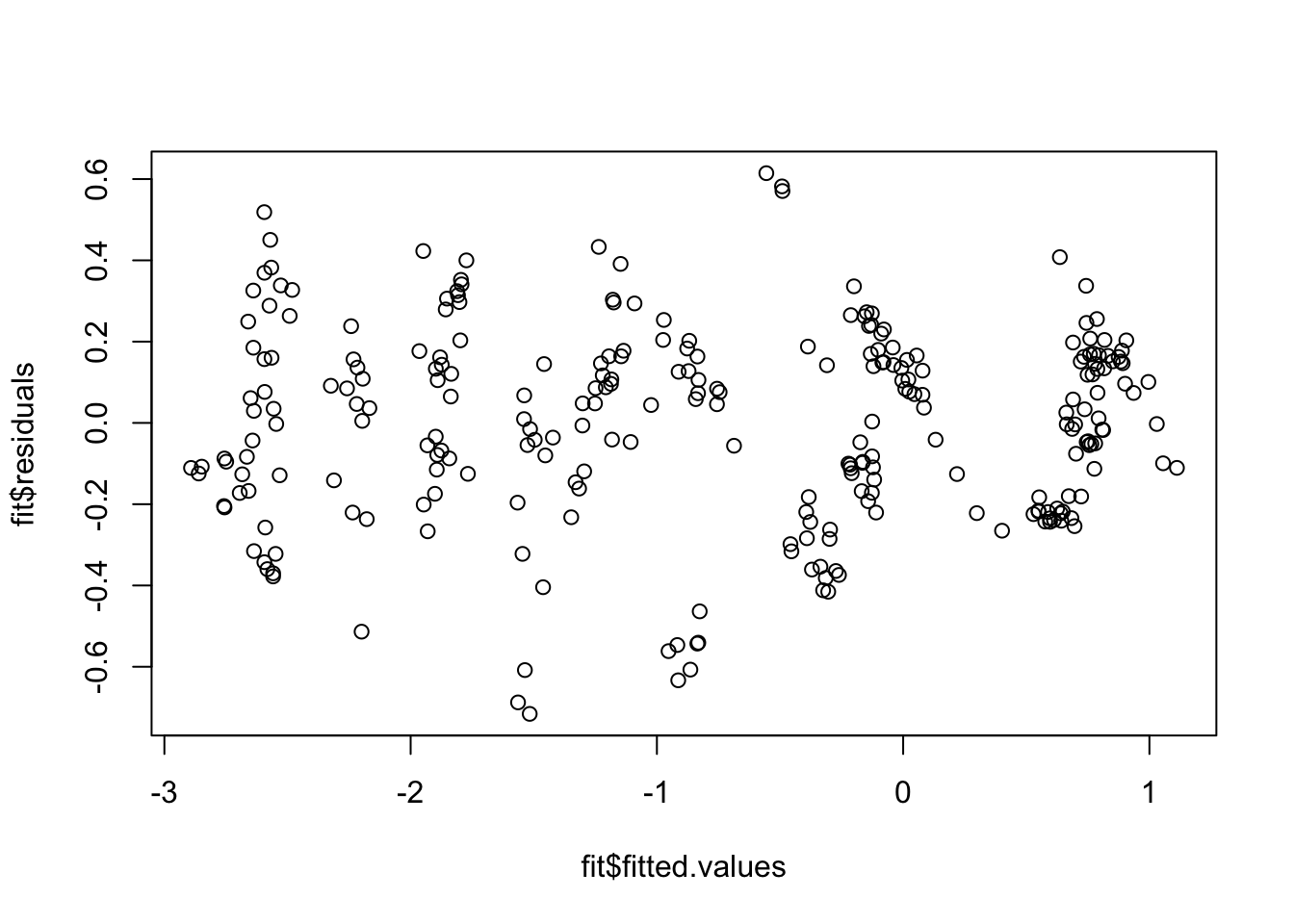
qqnorm(fit$residuals)
qqline(fit$residuals,col = "red")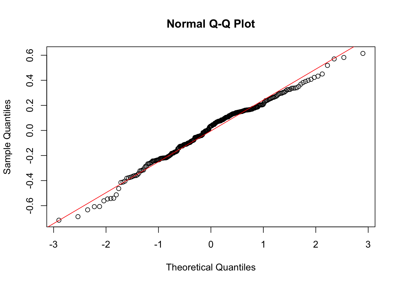
The second plot, of the fitted values and the residuals, might look a little suspicious. It does appear that there are some patterns present. One way to investigate this further is to colour the points by the category. We see that the categorical variable explains much of this pattern. Within each of the categories the residuals look quite reasonable and this is supported by the Normal-Quantile plot also. This is a good example of how some other factors can explain a potential pattern in the residuals which is actually not a concern.
plot(x = fit$fitted.values, y = fit$residuals, col = as.factor(Caterpillars$Instar))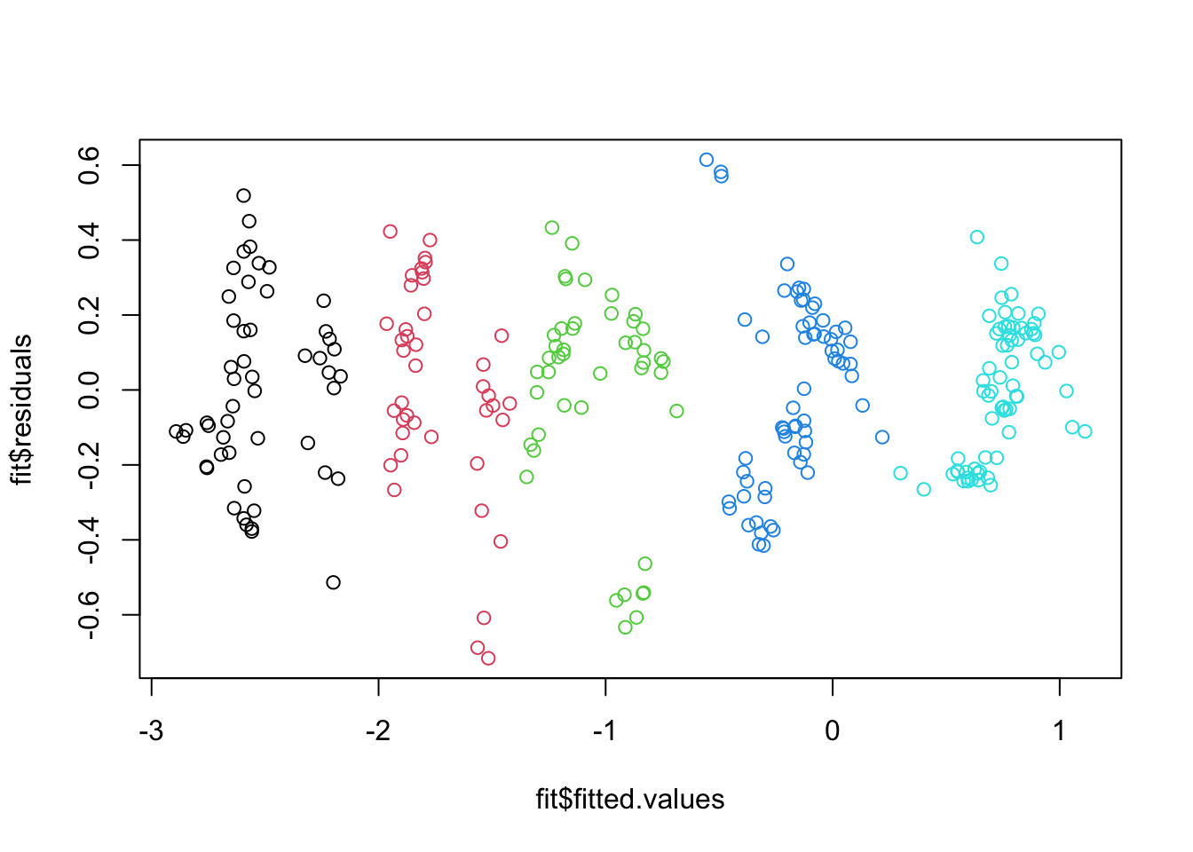
We will spend some time interpreting this regression fit. For this example, we have a binary variable and a categorical variable and we have a varying intercept for each.
The fitted model is therefore
\[ Y = \beta_0 + \beta_1 X_1 + \beta_2 X_2 + \beta_3 X_3 + \beta_4 X_4 + \beta_5 X_5 + \beta_6 X_6 + \epsilon, \]
where we have
- \(X_1\) is
LogIntake, a numeric variable - \(X_2\) is
as.factor(Instar)2, an indicator for whether the caterpillar is in the second stage of its life - \(X_3\) is
as.factor(Instar)3, an indicator for whether the caterpillar is in the third stage of its life - \(X_4\) is
as.factor(Instar)4, an indicator for whether the caterpillar is in the fourth stage of its life - \(X_5\) is
as.factor(Instar)5, an indicator for whether the caterpillar is in the fifth stage of its life - \(X_6\) is
ActiveFeedingY, an indicator for whether the caterpillar is actively feeding.
So we have a categorical variable with \(K=5\) possible categories, a binary variable and a continuous variable as our predictors. We are considering a varying intercept for each of the categories and the binary variable. We need \(6\) coefficients to encode this, as \(K-1=4\), \(1\) for the binary variable and \(1\) for the numeric variable. So our regression has \(p=6\).
Lets consider how we can have the different possible types of caterpillars in this model.
If we have a caterpillar which is not actively feeding and is in the first stage of life then we have \(\beta_2=\beta_3=\beta_4=\beta_5=\beta_6=0\) giving
\[ Y = \beta_0 + \beta_1 X_1 + \epsilon \]
If we have a caterpillar which is not actively feeding and in the second stage of its life then we have \(\beta_2=1\) and \(\beta_3=\beta_4=\beta_5=\beta_6=0\) giving
\[ Y = \beta_0 + \beta_2 + \beta_1 X_1 + \epsilon \]
Similarly, if we have a caterpillar which is in the 4th stage and actively feeding then we have
\[ Y = \beta_0 + \beta_4 +\beta_6 +\beta_1 X_1 + \epsilon. \]
So putting all the possible models together (which we have not shown here), we can interpret the coefficients as:
\(\beta_0\) as the average value of \(Y\) when \(X_1=0\) and a caterpillar is in the first stage and not actively feeding
\(\beta_1\) as the average increase in \(Y\) when \(X_1\) increases by 1 unit, holding all other predictors fixed.
\(\beta_2\) is the average change in the intercept in going from the first stage to the second stage of life, holding everything else fixed.
\(\beta_3\) is the average change in the intercept in going from the first stage to the third stage of life, holding everything else fixed.
\(\beta_4\) is the average change in the intercept in going from the first stage to the fourth stage of life, holding everything else fixed.
\(\beta_5\) is the average change in the intercept in going from the first stage to the fifth stage of life, holding everything else fixed.
\(\beta_6\) is the average change in the intercept in going from not actively feeding to actively feeding, holding everything else fixed.
What would an \(F\)-test mean for this regression? Remember that an \(F\)-test has a null hypothesis of \(H_0:\beta_1=\beta_2=\ldots =\beta_p=0\) vs the alternative that at least one of \(\beta_1,\ldots,\beta_p\) is not zero at \(\alpha = 0.01\), for example. So this \(F\)-test is testing whether there is a relationship between the log Mass of a Caterpillar and the predictors in the regression model. Based on the \(p\)-value in summary we would reject \(H_0\) at significance level \(\alpha\).
When you are using this in practice, and you use
varorsdinR, it actually divides by \(n-1\) rather than \(n\).↩︎