1 Recap

Before getting to the main components of this class, we will first spend some time reviewing material you have (hopefully) seen previously.

The language of statistics can be frustratingly precise and so we will review some of the terms you need to know here, before looking at some common examples of statistical analysis.

1.1 What does statistics do?

Broadly, statistics allows us to quantify uncertainty, to know something about a process which has some randomness built into it. We can never fully know everything about this randomness, but statistics allows us to get a handle on it at least. This normally consists of constructing a model for the process describing some data and evaluating that model.

A historic example, ending Polio

One historic example is the development of the first Polio vaccine in the 1950’s (Tanur and Lehmann 1985). A subset of the data from this study is shown below.

       Group Population Paralytic
1 Vaccinated     200745        33
2    Placebo     201229       115

It seems quite clear that less people became Paralytic among the group who received the vaccine, but how can we say this with any certainty? To do that, we need to use the language of probability and statistics.

There are multiple steps involved in going from proposing a scientific question to answering it with statistics.

We will give an outline for that process in this context and will highlight important concepts as we go along.

What is a model?

A statistical model is essentially just a way of describing data. It allows us to answer questions with data. For example, a model could help us answer the question: Are you more likely to get Polio if you don’t get vaccinated for it?

Very generally, a model is of the form

\[ Y = f(X) + \epsilon. \]

There are a few different things we can do with this formulation.

We can consider what general types of $f$ might make sense for our data.
We can estimate $f$, given that we have chosen a specific type.
Given we have estimated $f$, we can try predict what $Y$ will be at a specific value of $X$
We can assess the fit of our model to data. Does the estimated value of $f$ make sense for the data we have? How do we decide that one model is better than another? How do we determine that it is a suitable description of the data we have, or the question we’re trying to understand?

In a model like this, $Y$ is called the response variable, the outcome we are interested in.

$X$, which may be more than one variable, are called the explanatory variables.

The $\epsilon$ is the error. We never have a perfect model, and statistics is concerned with understanding what this error looks like. One way of seeing if your model is good is seeing what the errors look like, or are they consistent with the model we have chosen to fit.

This is vague at the moment but we will soon see specific examples below, which will help to make it much clearer.

The model fitting process

The model fitting process can be summarized as:

Choose a model
Fit the model to data
Assess the fit of the model for that data
Use the results from the model to understand the data

Note that you have to do a few things before you get to the model fitting process. You have to establish what question you are interested in, and you have to figure out what type of data could be used to answer this question. Then you have to actually collect this data. We will discuss these aspects below.

1.2 Key statistical concepts

We will first highlight two key questions considered by statistics:

Inferential statistics allows us to infer something unobservable. For example, how much would someone’s income increase if they got a college degree. Or, are you more likely to get Covid (again) if you don’t get vaccinated (again).

Predictive statistics allow us to estimate future or unknown quantities. For example, how much can you expect to make 5 years after taking this class?

The types of variables/data you have will influence how you can analyse the data

Data and Variables

The data given above about the Polio vaccine is a summary of the raw data, which would look something like this

# A tibble: 4 × 2
  Group      Paralytic
  <fct>      <fct>    
1 Vaccinated No       
2 Placebo    No       
3 Placebo    Yes      
4 Vaccinated No

Here we have multiple rows of data, with each row being a single observation (a person in the study). For each row we observe two pieces of information: whether they received the vaccine or not (the Group column) and whether the became paralytic or not (Paralytic column). These are the variables in the data.

The other output

The other text is part of the output from R, which we will explain as we go along. A tibble is just a data format which allows us to analyse the data easily. The <fct> tells us what type of variables Group and Paralytic are (categorical, see below).

Data is commonly arranged this way, where each row is an observation (or case or experimental unit), and each column is a variable.

These variables can only take on two values. You either get the vaccine or you don’t, and you either are paralytic or you aren’t. A variable which can only take on two values is a binary variable.

We can have lots of different types of variables.

Here is an example of some completely different data, about penguins in Antarctica, which has the same format, but different types of variables.

# A tibble: 6 × 4
  species island    bill_length_mm bill_depth_mm
  <fct>   <fct>              <dbl>         <dbl>
1 Adelie  Torgersen           39.1          18.7
2 Adelie  Torgersen           39.5          17.4
3 Adelie  Torgersen           40.3          18  
4 Adelie  Torgersen           NA            NA  
5 Adelie  Torgersen           36.7          19.3
6 Adelie  Torgersen           39.3          20.6

We have a species variable, telling us which species each penguin is. This is a categorical variable as there are only several possible species. The island variable is similar. Some categorical variables may have an ordering also (and are then ordinal). If they don’t have an ordering then they are called nominal variables.

Similarly, we have bill_length_mm, describing the length of a penguins bill. This is a quantitative variable, in that its a numeric value. These variables can be continuous, such as measurements, or discrete, such as years.

Note that we have NA in one of the rows. This is missing data, a frustrating but common problem which occurs if you ever try to collect real data. We will see this more later (and how to deal with it), but it’s important to be aware that it can happen!

There is one key difference in how these two datasets were collected. For the Polio data, this was a large (one of the largest ever at the time) experiments. The researchers who were investigating the effect of the vaccine designed the experiment so that they constructed the explanatory variable. It was decided before any data was collected who would get a vaccine and who wouldn’t. This is also known as a randomized experiment. The decision of who gets a vaccine and who gets a placebo is done in a careful (and safe) way, to ensure we can understand the effect of the vaccine. Randomized experiments make it easier to do causal inference, which lets us understand the causal effect of a treatment (here, the vaccine). That is we can ask: Does getting a vaccine cause less people to get polio?

For the penguin data, the researchers didn’t have the ability to assign penguins to different groups. They were simply observed in the wild and their data was collected. This is called observational data. This is much more common, and much easier to collect. However, it can be much harder to answer certain (important) questions with this data. Because we cannot assign penguins to a specific island, we can’t answer causal questions like: “Does living on a certain island cause penguins to have longer flippers?”. Instead, we can look at the association between these variables. For example, we can examine if there is a relationship between island and flipper length, but we cannot say that longer flippers is caused by living on a specific island.

Given a dataset, we can split the variables into groups based on the scientific question we’re interested in.

For the Polio example, we are interested in whether people will become paralytic, so this is the response variable, the outcome we are interested in. This is also called the primary variable.

All other variables are called explanatory variables. These are also called predictors or the independent variables or the covariates interchangeably. We will try to stick to only using one name in this class, but be aware that the other names are used.

1.3 Summarizing Data

While looking at the raw data is often important to explore and understand properties of the data, we often want to summarize the data in a more compact way.

How we summarize the data will depend on what properties of the data we think are important.

For example, we could use a numeric summary of the data to capture some overall general properties, while a graphical visualisation may be more useful to capture other properties.

Numeric Summaries

For the Polio data, we could summarize the raw data by simply getting the counts of how many people who got the vaccine were Paralytic and how many weren’t. This is because we are only considering two variables which can only take on two values each. So there are only 4 possible values for each observation.

But what can we do if we want to summarise the weight of a penguin? Counting all the penguins who weigh 3751g or 3254g maybe doesn’t make much sense. This would lead to a massive table, not a useful summary.

For numeric data we often want to reduce the amount of information we have to consider. If we have the weight of several hundred penguins, and we want to give someone a general summary that describes this data, we want to reduce this down to considerably fewer numbers.

We are often interested in reducing this information down to one or two numbers which capture important properties of the variable.

The maximum reduction in information would be to use a single number to summarise this variable. There are several possibilities, but one commonly used is the average, also known as the mean.

If we have weights $x_1,x_2,\ldots,x_n$ then this is computed by \[ \bar{x} = \frac{1}{n}\sum_{i=1}^{n}x_i \]

If we wanted to ask “Do male Adelie penguins weigh more than female Adelie penguins?”, we need to be able to compare these numbers.

We could get the mean of each (don’t worry if the code is unfamiliar)

Code

penguins %>%
  filter(species == "Adelie") %>%
  group_by(sex) %>%
  drop_na() %>% 
  summarise(avg_weight = mean(body_mass_g))

# A tibble: 2 × 2
  sex    avg_weight
  <fct>       <dbl>
1 female      3369.
2 male        4043.

An alternative one number summary of data such as this would be the median weight.

The median splits the data in half, such that 50% of the data is less than that value and 50% is greater than it.

In general this is not equal to the mean value. The median is less influenced by outliers, a small number of values which are very different to the majority of the data.

What if a single variable is not enough? For example, we could have two datasets which have the same mean but are vastly different.

For example consider the simple datasets \[ x = \{0,0,0,0,0,1,-1\}, y = \{4,-10,-10,10,6,5,-3,-2\}. \]

The mean of of both these datasets is 0 but at the same time they are very different. Simply saying they have the same mean is not really sufficient. We need a more informative summary.

To do this we need to consider further properties of the data, such as the variance.

This is closely related to the mean, captures how the data is spread about the average value, often using the notation $\sigma^2$ for the true value. We use $s^2$ for an estimate of the variance based on data (sample variance).

\[ s^2 = \frac{1}{n}\sum_{i=1}^{n}(x_i - \bar{x})^2 \]

Note: This is always a non negative number.

Can also consider $\sigma =\sqrt{\sigma^2}$, known as the standard deviation, and $s=\sqrt{s^2}$, the sample standard deviation, the number we would get from a sample of data.

For the above example, the $x$ data has variance 0.333 while the $y$ data has variance 55.71.

Note that for small data it is easy enough to compute these statistics by hand, but when we have real data (eg, 350 penguins), you want to use a computer to do these things.

mean(penguins$flipper_length_mm, na.rm = TRUE)

[1] 200.9152

var(penguins$flipper_length_mm, na.rm = TRUE)

[1] 197.7318

sd(penguins$flipper_length_mm, na.rm = TRUE)

[1] 14.06171

median(penguins$flipper_length_mm, na.rm = TRUE)

[1] 197

Missing Values

If we try to take the average of data where any entries are missing, R will return NA. We are removing the missing values here using na.rm = TRUE. In general, you should be careful doing this. You need to be sure that there is no reason that certain values are missing which could influence your scientific results.

A related notion of the variability of data is the Inter Quartile Range (IQR), which is based on percentiles of the data.

The 25th percentile, or first quartile, is a number $Q_1$ such that 25% of the data are less than that number.

The 75th percentile, or third quartile, is a number $Q_3$ such that 75% of the data are less than that number.

Then, the IQR is \[ IQR = Q_3 - Q_1 \]

A large IQR value indicates larger variability in the data.

More Variables

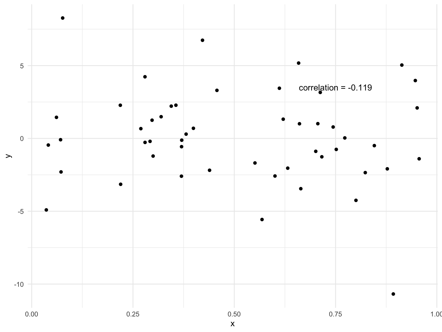
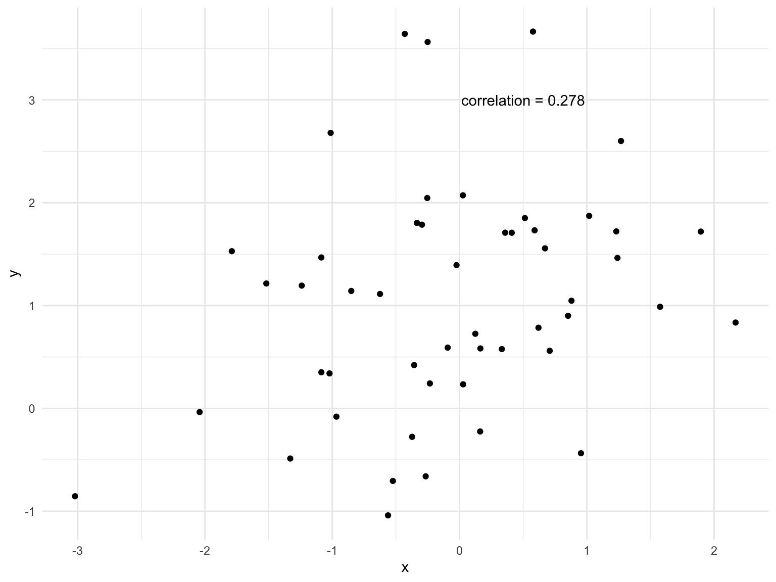
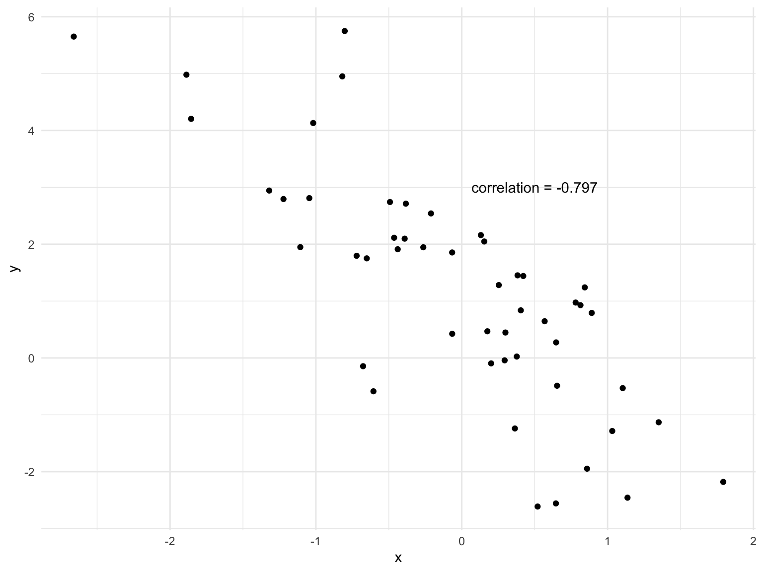
All the numeric summaries we have seen so far deal with a single variable. What if we want to summarize something more complex, such as the relationship between the height and weight

Want a numerical way of quantifying the relationship between two variables.

One statistic which has been developed to do this is the covariance between two variables, where for $x_1,x_2,\ldots,x_n,y_1,y_2,\ldots,y_n$ the sample covariance is

\[ cov_{x,y} = \frac{1}{n}\sum_{i=1}^{n}(x_i-\bar{x})(y_i-\bar{y}). \]

This can take on positive and negative values.

We can also look at the correlation of variables $X,Y$ where \[ corr_{x,y} = \frac{cov_{x,y}}{s_x s_y}. \]

This is the covariance divided by the individual standard deviations. This scales the covariance so that we always have $-1 \leq corr_{x,y} \leq 1.$

Covariance and correlation will always have the same sign.

We can compute the correlation between the body mass and flipper length of the penguins.

Code

penguins %>%
  drop_na() %>% 
  summarise(cor_mass_flip = cor(body_mass_g, flipper_length_mm))

# A tibble: 1 × 1
  cor_mass_flip
          <dbl>
1         0.873

Correlation just means there is some relationship between two variables, it doesn’t tell you if there is a causal relationship (see above).

Graphical Summaries

Instead of trying to reduce all the information for one variable down into one or two numbers, we could instead visualize the data as a way of summarising it.

While this is not as succinct as using the mean and variance, it provides vastly more information and can help to identify important components of the data.

Visualizations can help identify problems with our data.
Visualizations are more informative than numeric summaries when we wish to summarise more variables or the relationship between multiple variables.

The simplest such example is a bar plot for categorical data, which is equivalent to a table.

For example, we can do a bar plot of the penguin species.

Code

ggplot(penguins) + geom_bar(mapping = aes(x = species))

A bar plot showing how many penguins are of each species.

Single continuous variable

For a single continuous variable we can construct a histogram of the data.

To do this we break the data into several bins and plot how many values occur in each bin. Note that how large the bins are will influence what this plot looks like.

This gives us a measure of the overall spread of the data. Can also be used to identify unusual values.

Code

ggplot(penguins, aes(body_mass_g)) +
  geom_histogram()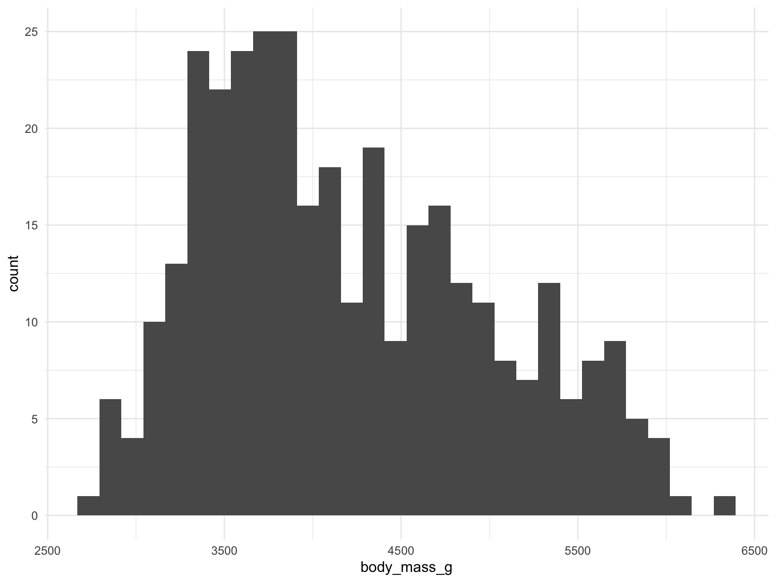

Code

ggplot(penguins, aes(body_mass_g)) +
  geom_histogram(bins = 50)

Changing the number of bins can make the histogram look quite different.

Similarly, we can compare the weight of male and female penguins by looking at a histogram for each.

Code

penguins %>%
  filter(species == "Adelie") %>%
  drop_na() %>%
  ggplot(aes(body_mass_g)) + 
  geom_histogram() +
  facet_wrap(~sex)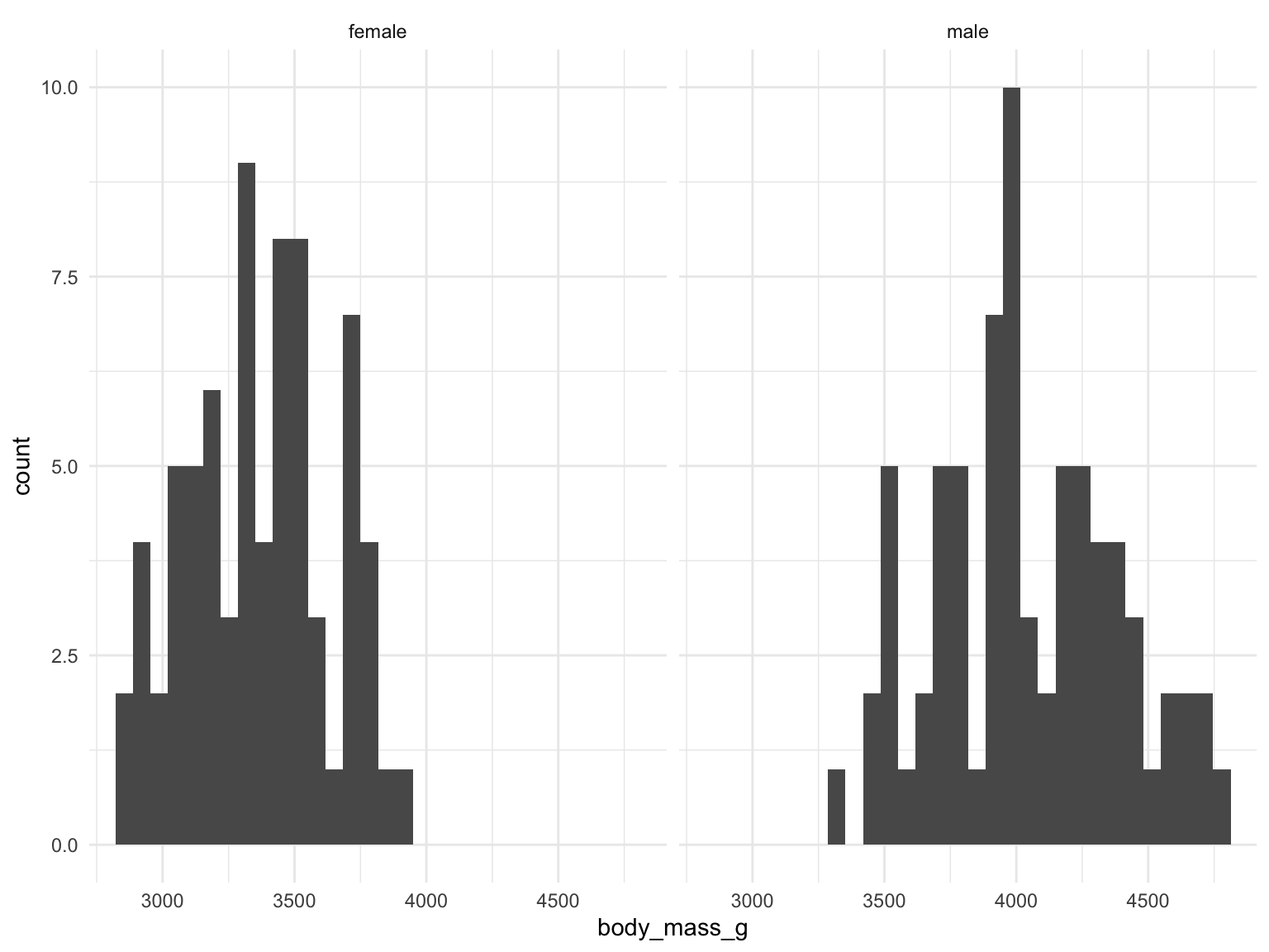

A histogram for male and female Adelie penguins.

Two Variables

For examining the relationship between two variables we can use a scatter plot (seen above), where we plot one variable on each axis and use a point to illustrate each observation.

This gives us some insight into how both variables vary together.

Code

ggplot(penguins, aes(bill_length_mm, bill_depth_mm)) +
  geom_point()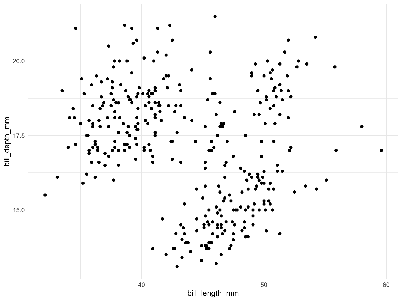

A scatterplot of bill length against bill depth.

Continuous and categorical

Often, we will want to explore these numeric relationships across some categorical groups. For example, we know there are multiple penguin species in this data. How can we include that in these plots?

Could create a separate plot for each species or indicate the different species on the one plot, eg using colour.

Let’s see what happens with the histogram.

Code

ggplot(penguins, aes(body_mass_g, fill = species)) +
  geom_histogram()

Showing the species on a histogram using colour.

For the histogram it is difficult to deal with the overlap in a single variable, so 3 separate plots might be clearer.

However, using colour works well for the scatterplot.

Code

ggplot(penguins, aes(bill_length_mm, bill_depth_mm, colour = species)) + 
  geom_point()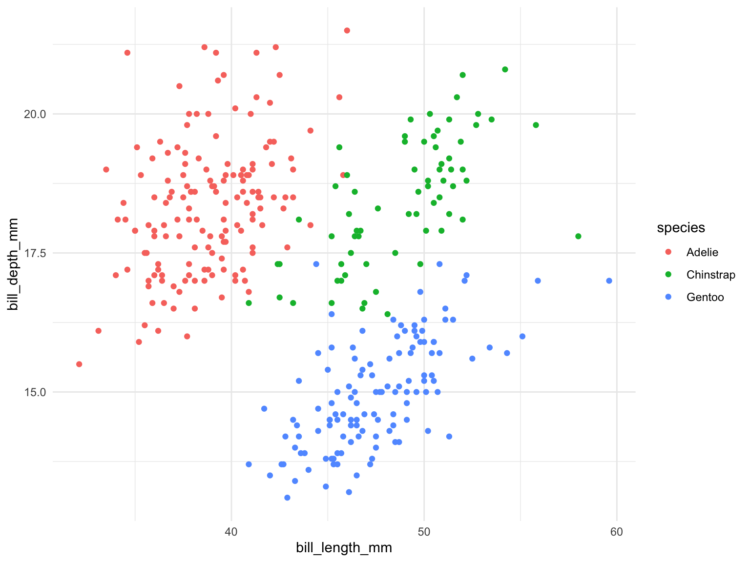

Colouring points in a scatterplot by species.

Visualizing data can be difficult and it is important to strike the balance between detail and clarity.

Samples vs Population

Given that we have some data, which we want to use to answer some question, the next step is figuring out what type of data we have, and what type of data we want to answer a question about.

Suppose we want to know something about the weight of all penguins in the world, such as, do male penguins weigh more than female penguins? Can we answer this with only the data we have collected, in penguins, which only contains a few hundred penguins?

# nrow is a function which tells us how many rows 
# of data we have.
# if organized properly, this will be the number 
# of observations
nrow(penguins)

[1] 344

The data we have is a sample from the population. This is a very common occurrence. We cannot catch and weigh every penguin, even with a lot of time and money. We need to be careful saying things about all penguins when we have only observed a few hundred on a few islands.

If our sample is sufficiently similar to the population, we might be ok. We need to see whether that is the case or not. If we can sample randomly from the entire population that is best, but it is often difficult.

The target population is the total population we want to learn about, such as all penguins or all students at SFU. The sample population is the population we actually collect data on, for example, all the penguins who could have been in this dataset. Or if our sample consisted of randomly picking 20 students in this class, the sample population would be all students in this class.

For example, for election polling, randomly calling numbers in the phonebook was long the gold standard. However, this has become less and less representative of the population of voters. Recently survey companies have tried to get random samples differently, including contacting Xbox users.

Random Sample

If you can get a true random sample of the population, you can be much more confident in trying to understand properties of the population than if you can only sample specific parts of the population. A true random sample means that every every observation in your target population has the same chance of being in your actual sample.

Parameters, Statistics

Given a question of interest, and some data from the target population, we want to know something about that population.

The population value of a variable is a parameter. We rarely know this, and we instead estimate it from our sample. Our estimate of a parameter from a sample is called a statistic.

Suppose the parameter we want to know is the average weight of all penguins. One potential estimate for this would be the average weight of the penguins in our sample.

mean(penguins$body_mass_g)

[1] NA

mean(penguins$body_mass_g, na.rm = TRUE)

[1] 4201.754

The variable we are interested in is random. We want to be able to quantify that randomness. Such as, what is the probability a penguin weights more than the mean? Or what is the probability a male penguin weighs more than a female one?

A random variable is a function which associates a number to each of the possible outcomes. The probability density function describes the values a random variable can take. This is also known as the distribution of a random variable. The pdf allows us to answer questions like: What is the probability a penguin weighs more than 5kg? We will pick a reasonable distribution for our data and try to estimate the parameters of that distribution. When we do that then we can use this to answer questions about our data.

Lets first see a simple example of a random variable.

Bernoulli Random Variables

Suppose we have a variable (which we will call $Y$) which can only take two possible values, i.e Yes (which we call $Y=1$) or No ($Y=0$). The Bernoulli distribution is a way to model this. For example, we are interested in understanding how many people have had Covid. We want to estimate the proportion of people who have had Covid. There are two options so this is a binary variable. The Bernoulli distribution is perfect for binary variables.

It says that $P(Y = 1) = p$ and $P(Y = 0) = 1-p$. These are the two possible values and the possible probabilities sum to 1. Thinking about our example, $p$ is the total proportion of all people who have had Covid.

Here $p$ is the parameter of the distribution. We want to try estimate this. We can think of $p$ as the proportion of times we would get $Y=1$ if we randomly generated a Bernoulli random variable many times.

If we observe data $y_1,\ldots, y_n$ then the proportion of these values which are 1 would be an estimate for $p$. Note that this is just the mean of the data we observe.

\[ \hat{p} =\frac{1}{n}\sum_{i=1}^{n}y_i. \]

The sample mean

We very regularly use the sample mean as our estimate for parameters because it has nice properties.

Upper and lower case

It can get a bit confusing that sometimes we use $X$ or $Y$ for data and sometimes we use $x$ or $y$. When we use upper case letters $X$ we are talking about data we have not observed, while as soon as we have actually observed the data then we use $x$.

The general procedure for using statistics to understand data is to choose a distribution for our data and then use that distribution. The most common and useful distribution is the normal distribution.

1.4 The normal distribution and some properties

This is the most well known and important distribution!

Can be used for real data taking on positive and negative values, such as in natural sciences where you measure quantities.

We say $Y$ follows a normal distribution with parameters $\mu,\sigma^2$ with pdf \[ f_{Y}(y) = \frac{1}{\sqrt{2\pi \sigma^2}}\exp\left( -\frac{1}{2\sigma^2}(y-\mu)^2 \right). \]

Here $\mu$ is the mean of the distribution, and $\sigma^2$ is the variance. The mean controls the average value the random variable will take while the variance controls how spread about the mean value the random variable is.

The normal parameters

People often write a normal distribution as $Y\sim\mathcal{N}(\mu,\sigma^2)$. We will use that convention here also, and everytime we do the second parameter will be the variance, not the standard deviation (the square root of the variance). Statistics can be confusing for switching between the variance and the standard deviation.

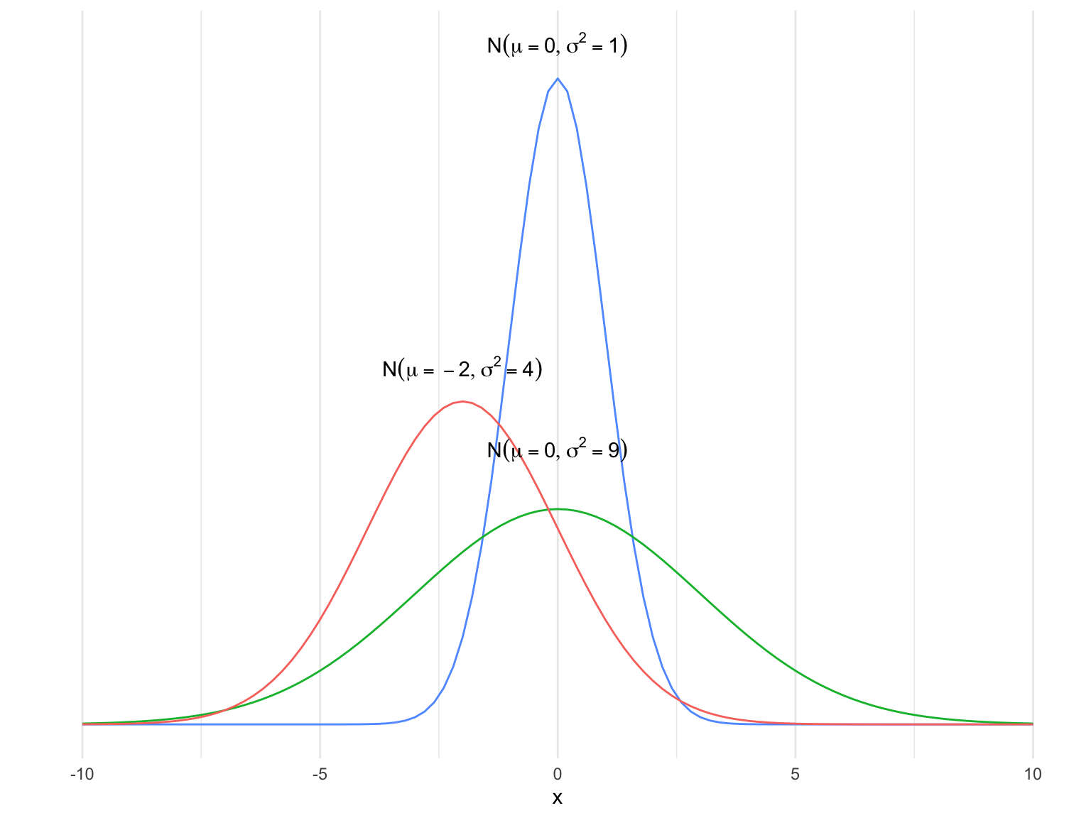
Some Normal pdfs

We can see that the normal distribution looks like a bell curve, with the mean parameter controlling where the center of the curve is, and the variance controlling how spread out around the center it is. The area under this curve is the probability a random variable from that distribution falls in the region under the curve. As this is a probability, the total area under any normal curve is 1. This means, for example, that if the probability a random variable is greater than 2.5 is 0.2, the probability it is less than 2.5 must be 0.8, because together they have to add up to 1.

Transforming to a standard Normal

If we have $Y\sim\mathcal{N}(\mu,\sigma^2)$ then

\[ Z = \frac{Y-\mu}{\sigma} \sim \mathcal{N}(0,1), \]

Doing this transformation is known as computing Z-scores, and are commonly used, because we know the properties of a standard normal.

For $Z\sim\mathcal{N}(0,1)$ then $P(Z\leq z) = \Phi(z)$, where $\Phi$ is a function that you can look up in a Z-table or ask R to compute.

Z-Scores

When do hypothesis tests and confidence intervals, we will often use values $z_{\alpha}$, where this means that for $Z\sim\mathcal{N}(0, 1^2)$ then $P(Z < z_{\alpha}) = 1-\alpha$. We will pick a value of $\alpha$ and want to determine the value of $z_{\alpha}$ which gives us a probability of $1-\alpha$.

How we will use this

This is extremely powerful, let’s explain what this means. If we had a variable which we know follows a normal distribution, we can compute the probability it will be in any specific interval.

For example, suppose $Y$ is how much your grade will differ from the class average on the final exam. If $Y$ follows a normal distribution with mean $0$ and variance $1$, then, you can compute the probability you get 1.5% below the average.

\[ P(Y < -1.5) = \Phi(-1.5) = 0.067. \]

The R code below computes the probability of getting a value smaller than -1.5 from a standard normal distribution. We will talk more about computing this shortly.

pnorm(-1.5)

[1] 0.0668072

We can do the exact same thing even for a variable which follows a normal distribution with a different mean and variance, by transforming to a standard normal. For example, suppose $Y$ is your percentage grade on the final exam, and $Y\sim\mathcal{N}(75, \sigma^2=100)$. What is the probability you will get a score greater than 82? We want to compute $P(Y>82)$. We will do this by transforming to a standard normal.

We know that

\[ Z=\frac{Y-\mu}{\sigma} = \frac{Y-75}{10}, \]

follows a standard normal distribution. We want to ask something about $Y$, but we will convert this into an equivalent statement about $Z$, making it easy to compute.

\[ P(Y > 82) = P\left(\frac{Y-75}{10} > \frac{82-75}{10}\right) = P(Z > 0.7). \]

To compute this, because the total probability has to be 1, we know that \[ P(Z>0.7) + P(Z < 0.7) = 1. \]

This means \[ P(Z > 0.7) = 1 - P(Z < 0.7) = 1 - \Phi(0.7). \]

We can compute this as above

1 - pnorm(0.7)

[1] 0.2419637

So we can now say $P(Y > 82) = 0.24$. These ideas will come up repeatedly in this class, so ensure they are familiar.

Standard Deviations from the Mean

We often want to know, for data from a normal distribution, how likely are we to see values far from the mean. If we have data from a $\mathcal{N}(0, 1^2)$ then the probability a random sample from this distribution is between -2 and 2 is \[ \Phi(2) - \Phi(-2) = 0.9544. \]

What this means is, if we can generate data from a normal distribution with mean 0 and variance 1, and we generate one point, the probability that that point is greater than -2 and less than 2 is more than 0.95. So if we did this 100 times, we would expect 95 of these data points to be between -2 and 2.

So over 95% of values within 2 standard deviations of the mean ($\sigma^2=1$ so we also have $\sigma=1$). To get exactly 95% use $z=1.96$, which we will see later.

We can write this as $P(-1.96 < Z < 1.96) = 0.95$.

Approximately 68% of values are within 1 standard deviation while 99.7% lie within 3 standard deviations. These approximations are often handy. For example, if we think we have data which follows a normal distribution and we observe a point which is more than 3 standard deviations from the mean, we know that this is quite unlikely to occur.

Connection to Hypothesis Testing

This is informally how hypothesis testing works. We will assume our data follows some distribution, and then by standardizing the data, this will correspond to a standard normal distribution. Then, if we get a value which is unlikely under a standard normal distribution, i.e more than 3 standard deviations from the mean, this is evidence our hypothesis might not be correct.

Symmetry of the Normal CDF

Because the normal distribution is symmetric about its mean value ($0$ here), the probability of getting a value smaller than $-2$ is the same as the probability of getting a value larger than $2$.

The area less than -2 under the curve is the same as the area under the curve to the right of 2.

Similarly, as we saw above we have that \[ P(-1.96 < Z < 1.96) = 0.95, \]

and because this is symmetric we have \[ P(Z < -1.96) = \frac{0.05}{2} = 0.025 = P(Z > 1.96). \]

So, using what we said above about defining $z_{\alpha}$, this means that

\[ z_{0.05/2} = z_{0.025} = 1.96. \]

Remember that $P(Z < z_{\alpha}) = 1 -\alpha$. We also know that \[ P(Z < -1.96) = 0.025, \] so this is the same as saying

\[ P(Z < -z_{0.025}) = 0.025. \]

So, for symmetric distributions (the normal distribution), we can put this together to say

\[ P(-z_{\alpha/2} < Z < z_{\alpha/2}) = 1-\alpha. \]

Common choices of $\alpha$ and $z_{\alpha/2}$ are:

$\alpha = 0.05$ which gives $z_{0.05/2} = 1.96$
$\alpha = 0.1$ which gives $z_{0.1/2} = 1.64$
$\alpha= 0.01$ which gives $z_{0.01/2} = 2.58$

We can also easily compute these using R.

alpha <- 0.05
qnorm(p = alpha/2, # the probability we want in the tail 
      mean = 0, # standard normal
      sd = 1, # standard normal
      lower.tail = FALSE) # TRUE would give us negative value

[1] 1.959964

Symmetric Data

If a distribution is symmetric then the mean will be equal to the median. The normal distribution and the t distribution (which we will see shortly) are symmetric.

Approximating using a Normal Distribution

It turns out that in many cases the normal distribution is a good approximation to other distributions, even non continuous ones. Suppose we have a Binomial distribution with 100 trials. This is the number of heads you get when you flip a coin 100 times, and we repeat that entire experiment many times. If we do a histogram of 1000 draws from that distribution, we see that…

The distribution of the number of times we get Heads tossing a coin 100 times, repeating this experiment 1000 times.

this looks quite like a normal distribution! Even, though the original data is counts between 0 and 100 and values of the normal distribution are continuous. This is in fact true for many types of data.

1.5 Central Limit Theorem

The previous example is true more generally. For almost all distributions, if you take a large sample $y_1,y_2,\ldots, y_n$ from that distribution, the mean of that sample,

\[ \bar{y} = \frac{1}{n} \sum_{i=1}^{n}y_i \]

is well approximated by a normal distribution.

So you compute things about the average of data from any distribution, once you know the mean and the variance of the distribution.

The central limit theorem says that if we have data $Y_1,\ldots, Y_n$ with mean $\mu$ and variance $\sigma^2$ then, as $n$ get larger and larger

\[ \frac{\sqrt{n}(\bar{Y}-\mu)}{\sigma} \]

becomes closer and closer to exactly $Z\sim\mathcal{N}(0, 1)$.

Sampling distribution

Suppose we have an estimate $\bar{y}$ of a random variable with mean parameter $\mu$.

The sample mean is an unbiased estimate for the population mean, which means that the long run average of the sample mean will be equal to the true value.

This estimate is an average of random variables

\[ \bar{Y} = \frac{1}{n}\sum_{i=1}^{n}Y_i, \]

so it also has a distribution! The distribution will depend on the distribution of the $Y's$.

If the $Y's$ come from a normal distribution $Y_i\sim\mathcal{N}(\mu,\sigma^2)$ then

\[ \bar{Y} \sim \mathcal{N}\left(\mu, \frac{\sigma^2}{n}\right). \]

So if we know $\mu$ and $\sigma$ then we know the distribution of $\bar{Y}$ exactly.

The mean of $\bar{Y}$ is $\mu$ which is another way of saying it is an unbiased estimate for $\mu$.

We can also then write that

\[ \frac{\bar{Y}-\mu}{\frac{\sigma}{\sqrt{n}}} \sim N(0, 1), \]

and so using what we had above about $z_{\alpha/2}$ for $Z$ a standard normal (which this now is), this tells us that

\[ P\left(-z_{\alpha/2} < \frac{\bar{Y}-\mu}{\frac{\sigma}{\sqrt{n}}} < z_{\alpha/2} \right) = 1-\alpha. \]

Sampling Distributions

This sort of formula is what we use over and over again for hypothesis testing and confidence intervals.

The t-distribution

We saw above that if we knew $\mu$ and $\sigma$ then

\[ \bar{Y} \sim \mathcal{N}\left(\mu, \frac{\sigma^2}{n}\right). \]

If we don’t know $\sigma^2$ we can estimate it with $s^2 = \frac{1}{n}\sum_{i=1}^{n}(y_i -\bar{y})^2$ for real data.

This changes the distribution of $\bar{Y}$ to a t-distribution.

\[ \frac{\sqrt{n}(\bar{Y} - \mu)}{s} \sim t_{n-1}. \]

This follows a t-distribution which now has a parameter $n-1$. This is known as the degrees of freedom of the t-distribution. For this $n-1$, the $n$ is the number of samples used to estimate $\bar{Y}$. Informally, because we have to estimate $s$, we lose a degree of freedom, hence we get $n-1$.

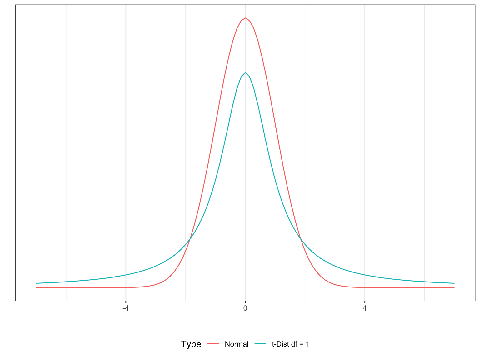
The t-distribution is similar to a normal but has more area in the tails. This means there is a larger probability of taking values far from the mean. Because we don’t know the variance and we have to estimate it, we have more uncertainty, which leads to the larger tails.

This has an important role when estimating parameters with real data.

The difference between the Normal and the t-Distribution

Much like with z-scores, we can also compute t-scores, such that for $\bar{Y}$ and $s$ estimated using a sample of size $n$ we have

\[ P\left(-t_{n-1, \alpha/2} < \frac{(\bar{Y}-\mu)}{\frac{s}{\sqrt{n}}} < t_{n-1, \alpha/2}\right) = 1-\alpha. \]

We call the denominator, $\frac{s}{\sqrt{n}}$ the standard error.

Here the value of $t_{n-1,\alpha/2}$ will change when $n$ changes. We can compute these using R.

alpha <- 0.05
n <- 100

qt(p = alpha/2, df = n - 1, lower.tail = FALSE)

[1] 1.984217

## if we have lower.tail = TRUE it will give us the negative of this value
qt(p = alpha/2, df = n - 1, lower.tail = TRUE)

[1] -1.984217

Notice that these t-scores are wider than the z-scores for the same $\alpha$.

1.6 Estimation

We have already seen a few examples of how we might estimate a parameter we don’t know.

If we want to estimate the mean parameter of a population, we use the sample mean for this. We saw that is has nice properties (unbiased).

\[ \bar{Y} = \frac{1}{n}\sum_{i=1}^{n}Y_i \]

We also saw that if we don’t know the variance of a distribution, we can estimate that also

\[ s^2 = \frac{1}{n}\sum_{i=1}^{n}(Y_i - \bar{Y})^2. \]

This will just give us a single estimate for the parameter. For example, if we get an estimate for the mean of the penguin weights,

mean(penguins$body_mass_g, na.rm = TRUE)

[1] 4201.754

We can’t then say that this is the mean population with much certainty. We know it might be a good estimate, but can we say more?

If we get an estimate of 4202g, is it possible that the true population mean is 1000g? What about 3500g? Is one more likely than the other? We saw above that we can say things about the distribution of the sample mean. We can then use that to say things about the population mean, if we have a good sample from the population.

1.7 Hypothesis Testing and Confidence Intervals

Hypothesis testing and confidence intervals are a rigorous framework for talking about the possible values an unknown parameter can take.

We have randomness here and so we can never say anything with complete certainty. There is a formal statistical language to express this which we will recap below.

Hypothesis testing allows us to testing whether a parameter take a specific value (such as, is the mean weight of penguins 4000g?) or a range of values (is the mean weight of penguins less than 3800g?).

Confidence intervals allow us to construct a range of plausible values for the parameter.

If we specify a test and a confidence interval in exactly the same way then the confidence interval will give you the same result as the hypothesis test, but only if specified equivalently.

We will start with some examples you will have seen before, using them to highlight the key components of testing and confidence intervals.

Confidence Intervals

To construct a confidence interval we are interested in finding a range of potential values for a parameter. A confidence interval for a parameter $\mu$ is some numbers $a,b$, based on $X_1,\ldots,X_n$, such that \[ P(a\leq \mu \leq b) = 1-\alpha, \]

for $\alpha$ close to 0, typically $\alpha = 0.1,0.05,0.01$. Here we will get values for $a$ and $b$, based on the data we have.

We saw that the sample mean of the weight of penguins was given by:

mean(penguins$body_mass_g, na.rm = TRUE)

[1] 4201.754

# get the number of observations 
# used to construct the mean
# total observations is 342
sum(!is.na(penguins$body_mass_g))

[1] 342

If the weights of penguins were normally distributed and we knew the variance, $\sigma^2$, then a $1-\alpha$ confidence interval would be

\[ \left( \bar{y} -z_{\alpha/2}\frac{\sigma}{\sqrt{n}}, \bar{y} +z_{\alpha/2}\frac{\sigma}{\sqrt{n}}, \right) \]

where $\bar{y}$ is the sample mean (mean(penguins$body_mass_g, na.rm = TRUE)), $\sigma$ is the known standard deviation, $n$ is the number of observations we used in computing $\bar{X}$ (sum(!is.na(penguins$body_mass_g))), and $z_{\alpha/2}$ is the value from the standard $z$ table such that there is area $\alpha/2$ in the tail beyond that value.

If we don’t know $\sigma$, then we have to estimate it, and our confidence interval becomes

\[ \left( \bar{y} -t_{n-1, \alpha/2}\frac{s}{\sqrt{n}}, \bar{y} +t_{n-1, \alpha/2}\frac{s}{\sqrt{n}}, \right) \]

where we now estimate the standard deviation with $s$ (sd(penguins$body_mass_g, na.rm = TRUE)) and because of this extra uncertainty, we have to use a $t$ distribution instead of a standard normal.

The t-Distribution

In practice, we will never know the population variance or standard deviation, and so will always be using the $t$ values instead of $z$ values.

We can compute this confidence interval in R.

bar_y <- mean(penguins$body_mass_g, na.rm = TRUE)
s <- sd(penguins$body_mass_g, na.rm = TRUE)
n <- sum(!is.na(penguins$body_mass_g))

## pick alpha = 0.05, so alpha/2 = 0.025 
t_val <- qt(0.025, n - 1, lower.tail = FALSE) 

lower <- bar_y - (s/sqrt(n)) * t_val
upper <- bar_y + (s/sqrt(n)) * t_val
c(lower, upper)

[1] 4116.458 4287.050

One Sided Confidence Intervals

Sometimes we only care about the interval in one direction. For example, for a new drug, we might only care if its better than existing treatments. Similarly, we might want to see if the proportion supporting a referendum is greater than 50%.

Now we won’t have $\alpha/2$ in both tails, will just have $\alpha$ in the tail that matters. So we will use $z_{\alpha}$ instead of $z_{\alpha/2}$

A lower confidence interval gives you a value $b$ such that

\[ P(\mu > b) = 1-\alpha \]

An upper confidence interval gives you a value $a$ such that

\[ P(a < \mu) = 1-\alpha. \]

For a lower confidence interval this gives you an interval

\[ \left(\bar{y} - t_{n-1, \alpha}\frac{s}{\sqrt{n}}, \infty \right). \]

For an upper confidence interval this gives

\[ \left(-\infty, \bar{y} + t_{n-1, \alpha}\frac{s}{\sqrt{n}}\right). \]

Example

To construct a 90% lower confidence interval for the mean weight of a penguin, we need to get $t_{n-1,0.1}$

t_val <- qt(0.1, df = n - 1, lower.tail = FALSE)
t_val

[1] 1.284039

bar_y - t_val * s/sqrt(n)

[1] 4146.072

This gives the interval

\[ (4146.072, \infty). \]

Properties of Confidence Intervals

Confidence intervals capture a range of values that are likely to contain the true unknown value. But it is not guaranteed! The upper and lower limits are based on the sample mean of the data which is random.

A 95% confidence interval means that if we got many many 95% confidence intervals, from many samples from the same population, we would expect 95% of them to contain the true value.

We say we have a ($1-\alpha$)% confidence interval. Common choices of $\alpha$ are 0.05, giving a 95% confidence interval and $\alpha=0.01$ giving a 99% confidence interval. A smaller $\alpha$ means a larger (wider) confidence interval (we have more confidence in it). Similarly, the width of the confidence interval will depend on $s$, larger $s$ gives a larger interval.

Hypothesis Tests

To do a hypothesis test, we need to come up with a hypothesis. In statistics, this is known as the null hypothesis. The null hypothesis is always the default or the norm being true, i.e that there is no difference in average blood pressure between the two groups.

We also have an alternative hypothesis, which is the hypothesis about the data we are interested in. For the drug example, the alternative hypothesis would be that the average blood pressure is lower in the group who receive the drug.

Informally, the idea of a hypothesis test is that we assume the null hypothesis is true and then, given that assumption, we investigate how likely the data we observed would occur under the null hypothesis. If there is little evidence, we will reject the null hypothesis.

To do this, one common technique is to perform a statistical test and obtain a p-value. A small p-value is seen as evidence that the null hypothesis is unlikely to be true. We will see a formal definition of the p-value later!

We mentioned above that if you don’t know the population variance you need to use a t distribution for your testing. In practice, this is always the case, and so it will be seen in all tests of the mean which follow.

Suppose we want to do a hypothesis test that the mean weight of penguins in our dataset is 4000g. When we do a test, we have randomness in our data and so somethings could go wrong:

We could conclude that the mean weight of penguins is not 4000g when it actually is. This is Type 1 Error.
We could conclude that the mean weight of penguins is indeed 4000g when this is not the case. This is known as Type 2 Error.

To do such a test we need to specify:

The null hypothesis. Here, this will be that the mean weight of the penguins $\mu = 4000$.
The significance level $\alpha$ at which we wish to test. This will control the Type 1 error. That is, we want probability we reject our null hypothesis when it is actually true to be $\alpha$.

The Significance Level

This has a big role on the outcome of your hypothesis test. You decide on $\alpha$ before you do the test. You cannot pick an $\alpha$, do a test and then redo the test with a different $\alpha$ to get statistically significant results. This makes your analysis invalid.

Then, to construct our hypothesis test we need to:

Construct our test statistics
Calculate the corresponding cut off from the $t$-distribution
Compare our test statistic to the cut off from the $t$-distribution, and determine whether we reject the null hypothesis or fail to reject it. If our test statistic is further from zero then the cut offs then we will reject the null hypothesis, otherwise we fail to reject.

Our test statistics will often be of the form (and for this section will always be similar to this)

\[ t = \frac{\bar{x} - \mu}{\frac{s}{\sqrt{n}}}, \]

where $\mu$ is the value of $\mu$ under the null hypothesis. If our null hypothesis is true, the $t$ should be a draw from a $t$-distribution with $n-1$ degrees of freedom. So if we get a value of $t$ which would be very unusual under that distribution (i.e, very far in the tails), then this is evidence that our null hypothesis is not true.

We first calculate our test statistic, which is the sample mean $\bar{y}$ minus the value of the mean under our null hypothesis (4000), divided by the standard error ($s/\sqrt{n}$).

bar_y <- mean(penguins$body_mass_g, na.rm = TRUE)
s <- sd(penguins$body_mass_g, na.rm = TRUE)
n <- sum(!is.na(penguins$body_mass_g))

test_stat <- (bar_y - 4000)/(s/sqrt(n))
test_stat

[1] 4.652499

Then, we need to calculate the cut off. This will depend on $\alpha$ and $n$, the number of samples.

## pick alpha = 0.05, so alpha/2 = 0.025 
## for more see ?qt
t_val <- qt(0.025, n - 1, lower.tail = FALSE) 
t_val

[1] 1.966945

Then we compare these. Because this is a two sided test (our null is $\mu=4000$) so our alternative is $\mu\neq 4000$, we need to check that our test statistic is greater than $-t_{val}$ and less than $t_{val}$. Otherwise we would reject.

-t_val < test_stat

[1] TRUE

test_stat < t_val

[1] FALSE

Therefore, because both of these conditions were not satisfied, we reject the null hypothesis at significance level $\alpha=0.05$.

We can also calculate a p-value here. Here we multiple by 2 because we are doing a two sided test.

p_value <- 2 * pt(q = test_stat, 
                  df = n - 1, 
                  lower.tail=FALSE)
p_value

[1] 4.69977e-06

Because the p-value is less than $\alpha=0.05$, this is an equivalent way of getting the same result.

The p-value is the probability of obtaining a test result as or more extreme than the one observed, if the null hypothesis was true .

The p-value is not the probability your null hypothesis is true! The definition is quite nuanced, and is very often misinterpreted.

What the p-value means is that, if the null hypothesis is true and we took many samples of size $n$ and each time constructed a test statistic, we would expect (for the penguin example where the p-value is 0.0000046) $0.0004\%$ of those test statistics to be larger than the one we observed, just by the inherent randomness. This is very unlikely, so it is evidence that the assumption of the null hypothesis being true is not reasonable, and we reject it.

A final comment is that p-values have been widely misused throughout scientific research, and understanding what they are and are not is very important for any statistical analysis.

Finally, note that even if we have evidence to reject the null hypothesis, it may not mean that the difference is practically significant. Suppose we determine that the mean of some quantity is not 4500g, but is likely to be a value very close to it, say 4510g. Does this 10g actually make a difference? This will depend on the problem!

Connection between hypothesis tests and confidence intervals

You might have noticed in the previous example that we used very similar calculations to get the confidence interval as to do the hypothesis test. They are equivalent, if specified in the same way.

Testing whether the mean $\mu=4000$ at significance level $\alpha =0.05$ is equivalent to getting a $1-0.05$ confidence interval for the mean and seeing if 4000 lies in the confidence interval you get. If it does not, you would reject the null hypothesis after performing the test.

For confidence intervals and hypothesis tests to agree we require:

The same significance level $\alpha$, for both
That the type of hypothesis test and the type of confidence interval agree. We will mostly use two sided confidence intervals, which match with testing whether the parameter is equal to a value or not, the example we did above.

1.8 More examples you may have seen before

One Sample Normal Mean

Lets do some more examples of testing a normal mean for some data. We will use some data from a large survey, which we can load into R.

gss

# A tibble: 500 × 11
    year   age sex    college   partyid hompop hours income class finrela weight
   <dbl> <dbl> <fct>  <fct>     <fct>    <dbl> <dbl> <ord>  <fct> <fct>    <dbl>
 1  2014    36 male   degree    ind          3    50 $2500… midd… below …  0.896
 2  1994    34 female no degree rep          4    31 $2000… work… below …  1.08 
 3  1998    24 male   degree    ind          1    40 $2500… work… below …  0.550
 4  1996    42 male   no degree ind          4    40 $2500… work… above …  1.09 
 5  1994    31 male   degree    rep          2    40 $2500… midd… above …  1.08 
 6  1996    32 female no degree rep          4    53 $2500… midd… average  1.09 
 7  1990    48 female no degree dem          2    32 $2500… work… below …  1.06 
 8  2016    36 female degree    ind          1    20 $2500… midd… above …  0.478
 9  2000    30 female degree    rep          5    40 $2500… midd… average  1.10 
10  1998    33 female no degree dem          2    40 $1500… work… far be…  0.550
# ℹ 490 more rows

We are interested in the average number of hours worked. Lets first see a histogram of this data.

Code

gss %>% 
  ggplot(aes(hours)) +
  geom_histogram() +
  labs(x = "Hours Worked in a Week", y = "Count")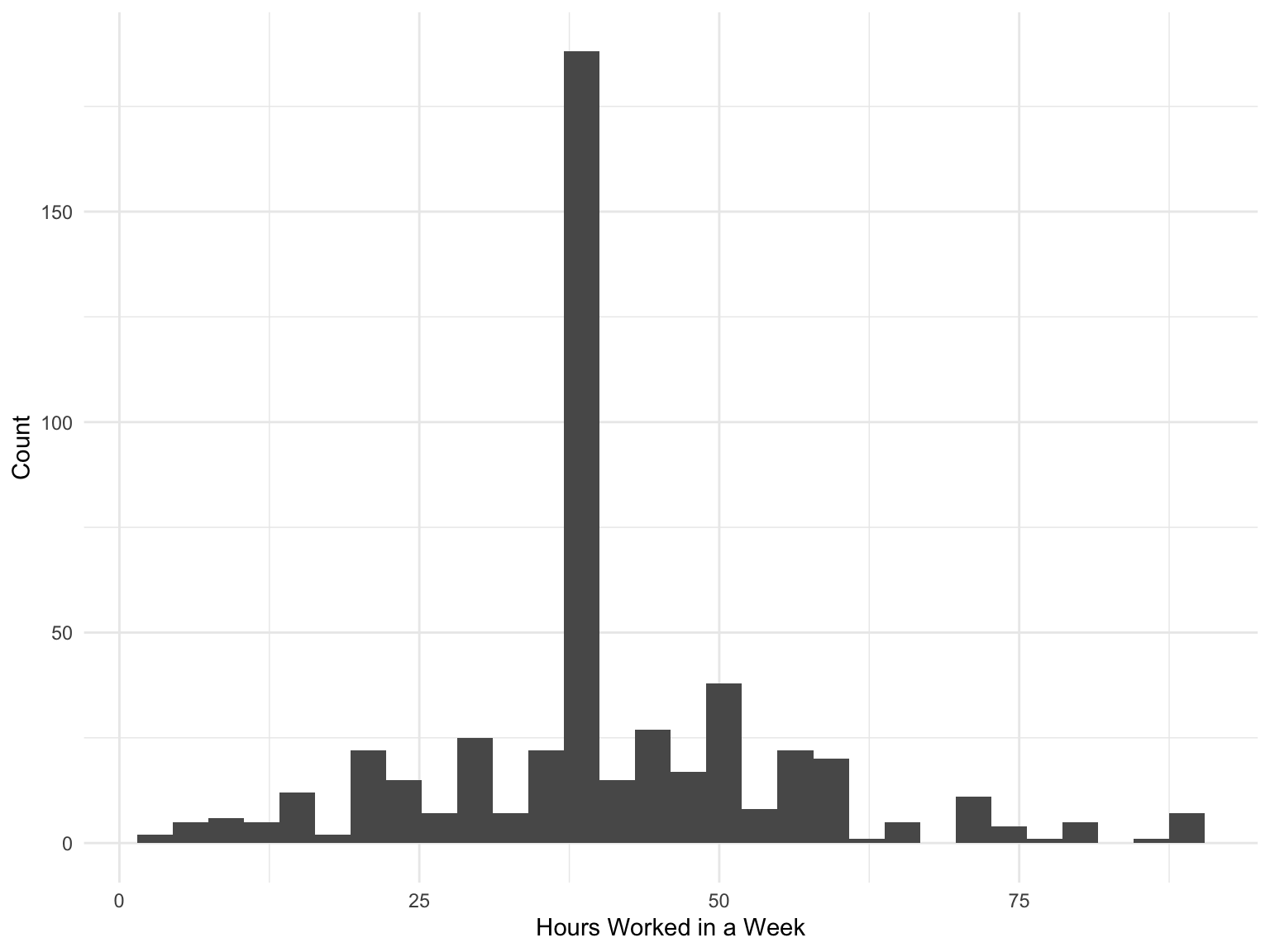

The data we are using for our hypothesis test.

Let’s do a hypothesis test on whether the average person in this study works 40 or less hours a week. We denote by $\mu$ the number of hours worked a week. Our hypothesis will be:

The null hypothesis, $H_0$: That $\mu \leq 40$
The alternative hypothesis, $H_A$: That $\mu > 40$.

We will specify $\alpha = 0.01$.

This is a one sided hypothesis test, so slightly different to the previous examples. Lets also construct the corresponding confidence interval. To do that we need to specify the conf_level, which is $1-\alpha=0.99$.

Note

To perform hypothesis tests we will use some functions in the infer package, which you will need to install using install.packages("infer").

t_test(gss, response = hours, 
       mu = 40, alternative = "greater", 
       conf_level = 0.99)

# A tibble: 1 × 7
  statistic  t_df p_value alternative estimate lower_ci upper_ci
      <dbl> <dbl>   <dbl> <chr>          <dbl>    <dbl>    <dbl>
1      2.09   499  0.0188 greater         41.4     39.8      Inf

Because our p-value, 0.0188 is (just) larger than our choice of $\alpha$, we fail to reject the null hypothesis. Similarly, because the corresponding confidence interval goes below $40$, this is equivalent to failing to reject the null.

One Sample Proportion

Another important example is comparing proportions. Suppose we want to examine the proportion of people in a population who have some characteristic.

For example, we could test whether the proportion of female penguins is equal to $0.5$ or not.

$H_0:p = 0.5$
$H_{A}:p \neq 0.5$

We choose $\alpha = 0.1$.

This test statistic is approximately normal and we can compute this in R using.

prop_test(penguins %>% drop_na(),
          ## need to remove missing values
          sex ~ NULL,
          ## specify the variable of interest
          success = "female",
          ## specify which is success
          p = 0.5,
          ## specify the null hypothesis
          z = TRUE) ## specify to do a z-test

# A tibble: 1 × 3
  statistic p_value alternative
      <dbl>   <dbl> <chr>      
1    -0.164   0.869 two.sided

Here the statistic is

\[ \frac{\hat{p} - 0.5}{\sqrt{\frac{\hat{p}(1-\hat{p})}{n}}}, \] where $\hat{p}$ is the proportion of penguins which are female. Under the null hypothesis this follows a $\mathcal{N}(0, 1^2)$ distribution.

Because our p-value is greater than $\alpha$ we fail to reject the null hypothesis.

A confidence interval can also be constructed but has been omitted here. It will be of the form

\[ \left(\hat{p}-\sqrt{\frac{\hat{p}(1-\hat{p})}{n}} z_{\alpha/2}, \hat{p}+\sqrt{\frac{\hat{p}(1-\hat{p})}{n}} z_{\alpha/2} \right). \]

Paired t-Test

More often we want to compare whether a parameter is the same across two (or more groups). There are several ways we can do this, depending on the type of data we have.

Quite often we might have some paired data. For example, suppose students take a standardised test and get the following scores. Then, they take a specialized training program and take the same test again. We want to see if the training made them do better, with the following scores, for the students in the same order

student_scores

# A tibble: 8 × 3
  students  init after
  <chr>    <dbl> <dbl>
1 student1    56    59
2 student2    43    48
3 student3    62    63
4 student4    59    57
5 student5    38    45
6 student6    61    64
7 student7    51    53
8 student8    47    49

Because each of the 8 students took the same test twice, we have a before and after value for each. We want to see if the before is equal to the after. We have a natural pair here (the two scores from each student), so we can look at the difference

difference <- student_scores$after - student_scores$init
difference

[1]  3  5  1 -2  7  3  2  2

The null hypothesis of this training not helping would be the same as saying the mean of these differences is 0. That is what we then test, with a t-test with $n-1$ degrees of freedom. We specify $\alpha = 0.05$.

student_scores$difference <- difference

t_test(student_scores, response = difference,
       alternative = "two-sided", 
       mu = 0, conf_level = 0.95)

# A tibble: 1 × 7
  statistic  t_df p_value alternative estimate lower_ci upper_ci
      <dbl> <dbl>   <dbl> <chr>          <dbl>    <dbl>    <dbl>
1      2.78     7  0.0272 two.sided       2.62    0.393     4.86

Because the p-value is less than $\alpha$ (or equivalently, because the interval doesn’t contain 0), we have evidence to reject the null hypothesis that there is no difference and based on the confidence interval, it does appear that the training leads to improve test scores.

Two Sample t-Test

The paired t-test needs some natural pairing to be present in the data, which is not always available. In other cases, we instead use a two sample t-test.

For example, suppose we look at the gss data again, and we want to compare the number of hours worked by those with a college degree vs those without a degree.

Code

gss %>% ggplot(aes(college, hours)) +
  geom_boxplot() +
  labs(x = "College Education", y = "Hours Worked")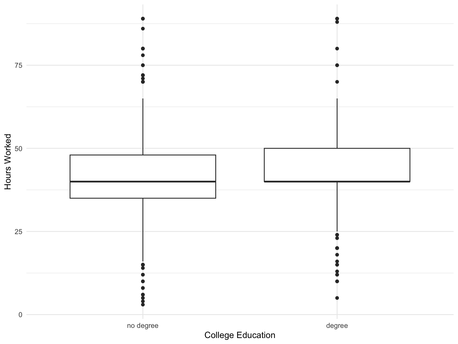

Boxplots

A boxplot is used for comparing continuous variables across different categories. The solid black horizontal line in the box shows the median, the top and bottom of the boxes show $Q3$ and $Q1$ and the lines extend $1.5 IQR$ from $Q3$ and $Q1$. Any points beyond this distance from the box are shown individually.

It looks like both groups work a similar number of hours, but we want to confirm this with a hypothesis test. We do this with a two sample t-test.

We have samples from two groups now, where we have a sample mean $\bar{x}_1$ in the first group and $\bar{x_2}$ in the second group. We have $n_1$ observations in the first group and $n_2$ in the second group. The population mean for group 1 is $\mu_1$ and the population mean for group 2 is $\mu_2$.

We want to test whether the mean of the first group is equal to the mean of the second.

Our null hypothesis is $H_0: \mu_1 = \mu_2$.

Our alternative hypothesis is $H_A: \mu_1 \neq \mu_2$.

There are several difficulties now compared to a one sample t-test that we saw before.

How do we estimate the sample variance?
What are the degrees of freedom?

An estimate for the pooled sample standard deviation is given by

\[ s_p = \sqrt{\frac{(n_1-1)s_1^2 + (n_2 - 1)s_2^2}{n_1 + n_2 - 2}}, \]

where $s_1$ is the sample standard deviation of the first sample and $s_2$ is the sample standard deviation of the second sample. $n_1$ is the number of observations in the first group and $n_2$ is the number of observations in the second group. This is valid when the standard deviation of the two groups is approximately the same. If not, we need to use a different estimate. We also still need to account for the number of samples in each group, $n_1$ and $n_2$.

The degrees of freedom is

\[ n_1 + n_2 - 2. \]

So our estimate is

\[ \frac{\bar{x_1}-\bar{x_2}}{s_p \sqrt{\frac{1}{n_1}+ \frac{1}{n_2}}}, \]

and this follows a t-distribution with $n_1 + n_2 - 2$ degrees of freedom.

We can do this test using R. Note that if we don’t specify var.equal = TRUE, it will use a slightly different formula to calculate the pooled standard deviation. In practice, you will probably get a similar result.

t_test(x = gss, 
       formula = hours ~ college, 
       order = c("degree", "no degree"),
       alternative = "two-sided", var.equal = TRUE)

# A tibble: 1 × 7
  statistic  t_df p_value alternative estimate lower_ci upper_ci
      <dbl> <dbl>   <dbl> <chr>          <dbl>    <dbl>    <dbl>
1      1.11   498   0.269 two.sided       1.54    -1.19     4.27

Here we use formula to specify that we want to test whether the number of hours worked varies across the value of college. The order would be important if we did a one sided test, picking which group is group 1 and which is group 2.

Similarly, we can get a confidence interval for the difference between two means, which will be of the form

\[ \left( (\bar{x}_1-\bar{x}_2) - t_{n_1+n_2 -2, \alpha/2}s_p \sqrt{\frac{1}{n_1}+ \frac{1}{n_2}}, (\bar{x}_1-\bar{x}_2) + t_{n_1+n_2 -2, \alpha/2}s_p \sqrt{\frac{1}{n_1}+ \frac{1}{n_2}} \right). \]

We can compute all these quantities in R once we know the sample means, sample standard deviations and the number of samples in each group.

1.9 Summary

Using statistics to study data relies heavily on making assumptions about the model you choose and the data you have. As such, it is important to check that these assumptions are reasonable. If the assumptions of a statistical model or a hypothesis test are completely unreasonable for some data, you should not trust your results.

In this section we’ve seen some common ways to construct hypothesis tests and confidence intervals. They mostly rely on the assumption that the data follows a normal distribution. However, because we don’t know the parameters of this normal distribution, when we estimate them it follows a $t$-distribution. So we assume our data follows a $t$-distribution, and then construct tests and confidence intervals based off of that assumption.

Following this section, you should be comfortable understanding different types of variables and have some knowledge of how data can be collected, and how this collection can impact the things you can say with your data. You should understand that hypothesis testing makes an assumption about the distribution of data and then sees how plausible the data you have is under that assumption.

You should be able to construct and interpret the confidence intervals and hypothesis tests shown in this section, given some data.

Thinking about the assumptions behind a model and checking if they are reasonable will come up again and again in this class.

1.10 Practice Problems

Below are some additional practice problems related to this chapter. The solutions will be collapsed by default. Try to solve the problems on your own before looking at the solutions!

Problem 1

A survey collected data about how much education individuals received and their annual income, along with the number of people in each group.

Education	average_Income	number
8th Grade	41666.67	7
9 - 11th Grade	40892.86	16
College Grad	73920.45	46
High School	46730.77	29
Some College	52434.21	42
NA	49811.32	60

Given the number of people in each group, comment on the people who didn’t reply to the Education question (the NA group).
Suppose you were interested in testing whether college grads have a different average income to high school graduates. Do you think the missing data could have an impact on this test?

Solution

For the first part, we can only base our answer on the data we have. The number of people who don’t answer the education question is large, and they have a smaller average income than those who went to college. Perhaps the people who didn’t answer the Education question are embarassed that they didn’t attend college.

For the second part, this missing data could have a big impact on this hypothesis test. If, hypothetically, all the people who didn’t answer the education question actually were high school graduates, they would significantly change the mean for that group. That could change the result of the hypothesis test, leading to a different result.

Problem 2

A machine is being constructed which aims to improve air quality in classrooms. Suppose we record the C02 levels in 15 classrooms, then place this machine in each classroom for a week, before again recording the C02 levels (in ppm).

The summary data is shown below, of the difference between the C02 before and after the machine was used:

Statistic	Value
n	15
$\bar{x}_{diff}$	10.45
$s_{diff}$	3.54

Explain the assumption required to use a paired t-test for this data, and why it is satisfied here.
Given you can treat this data as paired, construct a 90% confidence interval for the difference in C02 after using the machine.

Solution

For the first part, to do a paired t-test, we need a natural pairing of the data. Here, we observe data in the same classroom a week apart. Because we have a pair of datapoints for each classroom, a paired t-test is appropriate here.

To construct this confidence interval, we need to compute the correct t value, which is $t_{15-1,0.05}=1.76$, because we have a 90% interval. This gives the following interval

$\left(\bar{x}-t_{n-1,0.5}\frac{s}{\sqrt{n}}, \bar{x}+t_{n-1,0.5}\frac{s}{\sqrt{n}}\right) = (10.45 - (1.76)\frac{3.55}{\sqrt{15}},10.45 + (1.76)\frac{3.55}{\sqrt{15}})$

Problem 3

A researcher wishes to examine the birth weight (in ounces) of babies born to first time mothers compared to babies born to mothers who have given birth previously. The perform a two sided two sample t-test at $\alpha = 0.05$, computing the mean weight of babies born to first time mothers, minus the mean weight of babies born to mothers who have given birth previously.

These results are shown below, along with a two sided 95% confidence interval for the difference.

# A tibble: 1 × 7
  statistic  t_df p_value alternative estimate lower_ci upper_ci
      <dbl> <dbl>   <dbl> <chr>          <dbl>    <dbl>    <dbl>
1      1.62  1234   0.105 two.sided       1.93   -0.405     4.26

Suppose instead the researcher had constructed a one sided hypothesis test, and was only interested in whether the mean weight was greater in babies born to first time mothers. How would the p-value change, if the significance level remained the same?
If the researcher had instead constructed a lower confidence interval for the difference, how would the confidence interval change? You do not need to compute anything for this part.

Solution

For a two sided hypothesis test, the p-value is the probability of getting a result as or more extreme in either direction. So the p-value corresponds to getting a test statistic greater than 1.62 or less than -1.62. If a one-sided test was performed instead, then the p-value would only correspond to getting a test statistic larger than 1.62, not the negative value. In that case, the p-value would be $0.105/2$.

For a lower confidence interval, the upper value would be $\infty$ and the lower value would be conputed similarly to the current two sided interval, but with a different t score, using $\alpha$ instead of $\alpha/2$.

Problem 4

A researcher is interested in understanding the average height of a group of adults, and whether it is 70 inches or not. A histogram of the data is shown below, along with a numeric summary of the data.

x_bar	s	n
68.311	1.848	928

Give one assumption required to do a hypothesis test for this data.
Perform a two sided hypothesis test of $H_0:\mu = 70$ vs $H_A:\mu\neq 70$ at significance level $\alpha = 0.01$.

Solution

Assumptions required to do this hypothesis test are that the data are independent and that the data can be approximated by a normal distribution.

For this hypothesis test the test statistic would be $t = \frac{68.311-70}{\frac{1.848}{\sqrt{928}}}=-27.84$. Here $\alpha=0.01$ for the critical value from the t-distribution is $t_{n-1,0.005}=2.58$. Since the test statistic is further from 0 than the critical value, we have evidence to reject the null at $\alpha=0.01$.