2 Simple Linear Regression
2.1 Setup
Very often we have more than one variable and we want to understand the relationship between these variables.
We saw very simple examples of this in the previous section, where we had two groups and we wanted to see if variables differed across groups. We used a two sample t-test to check this. Now we want something more general.
Perhaps surprisingly, a line can often describe the relationship quite well, if not exactly. In any case, its a good starting point.
This is related to the idea of correlation we saw back in Chapter 1.
Example
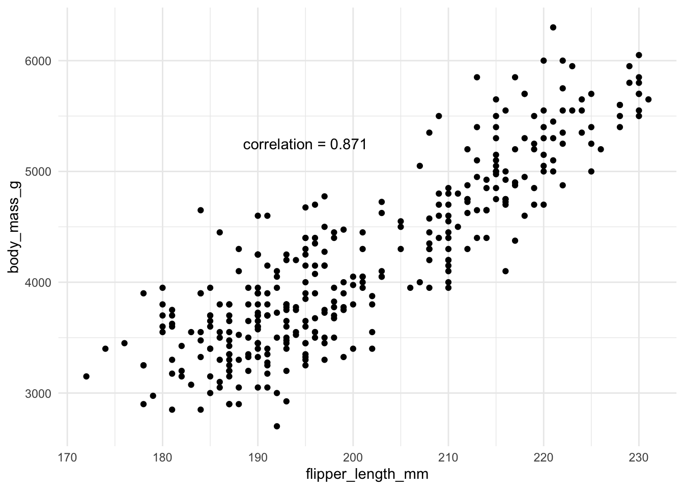
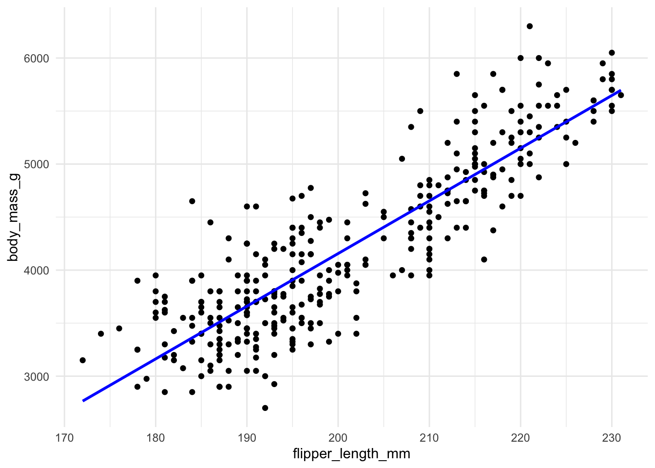
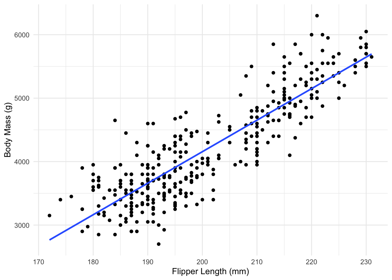
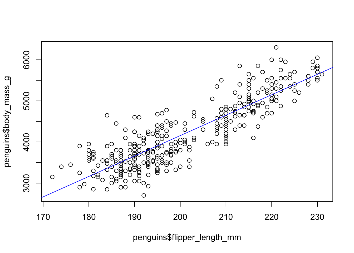
Here is an example using the penguin data again and the relationship between flipper length and body mass, which appears to be quite linear. As a penguin’s flippers get longer, it seems, on average, that they weigh more too, and that this relationship is somewhat linear.
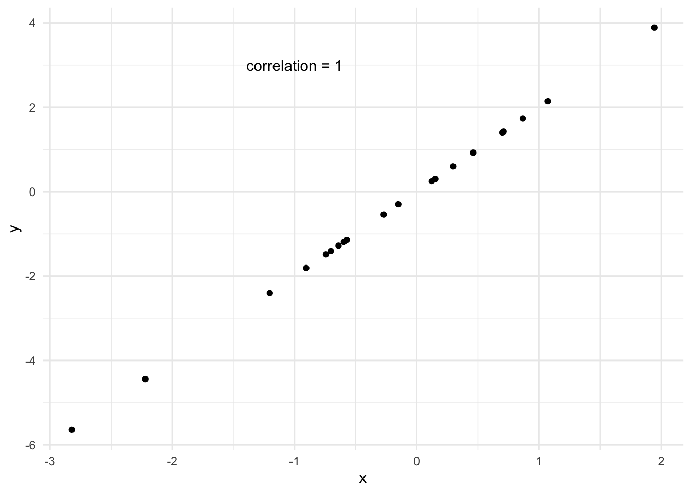
If the correlation is exactly 1, then a straight line fits the data perfectly. But that is rarely ever the case with real data.
We want to fit the best line possible in the case where the data is not perfectly linear but a straight line is a good approximation. This goes back to the idea of a model. We are proposing a model for our data, and checking if it is a good approximation.
Very generally, we said our model looks like
\[ Y = f(X) + \epsilon, \]
With a linear model, we are choosing a specific type of \(f\).
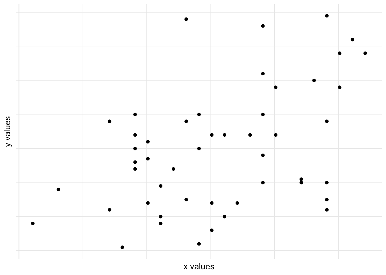
No single line can be used which will be perfect for the real data above. No one line will go through all the data, it will always miss some of the points.
To pick a “best” line, we have to define what we mean by a “good” fit.
First of all, how do we define a straight line? We need to know two things: The intercept (\(a\)) and the slope (\(b\)).
Once we know both of these and some values of \(x\) coordinates, we can easily compute the values of \(y\), using
\[ y = a + bx, \]
and draw the line.
2.2 Linear Regression Equation
Linear regression is just saying this in a slightly different way, and accounting for the fact that real data will not follow a line exactly. We use an equation of the form
\[ y = \beta_0 + \beta_1 x +\epsilon. \] This is exactly how we wrote a general model, with
\[ f(x) = \beta_0 + \beta_1 x. \]
Here \(\beta_0\) is the intercept of the line, the \(y\) value of the line when \(x=0\).
\(\beta_1\) is the slope of the line.
\(\epsilon\) is the error of the line, the distance from the line to each point. If all our data lay on a straight line then we could have \(\epsilon=0\), but real data is never like this.
We call \(x\) the explanatory or predictor variable. The value of \(x\) should give us some information about the value of \(y\), if our line describes the data. If our line has a positive slope, then as we increase \(x\) we expect \(y\) to increase. Similarly, if we have a negative slope, as we increase \(x\) we expect \(y\) to decrease.
We call \(y\) the response variable. This model also assumes that the true errors, \(\epsilon\) are normally distributed, with mean 0 and some variance \(\sigma^2\), \(\epsilon \sim \mathcal{N}(0, \sigma^2)\). This is a key assumption for fitting a linear regression and we will spend a lot of time investigating it below.
Fitting a linear regression
Suppose we have a line which we use to model the data, which we will call
\[ \hat{y}_i = \hat{\beta}_0 + \hat{\beta}_1 x_i. \]
Notation
Whenever we use a hat, i.e \(\hat{\beta}_0\), we are talking about an estimate of a parameter, or when we use \(\hat{y}\) then we are talking about the estimate of \(y\) using \(\hat{\beta}_0\) and \(\hat{\beta}_1\).
What this says is that for each \(x_i\) our line gives an estimate of \(y_i\), \(\hat{y}_i\), which is the corresponding \(y\) coordinate on the line with intercept \(\hat{\beta}_0\) and intercept \(\hat{\beta}_1\). This is called the fitted value
The line does not need to go through any of the actual points so normally \[ \hat{y}_i \neq y_i \]
We say the distance between the true point and the line is the residual, the difference between the observed \(y\) value and the estimated \(y\) value, for the same value of \(x\).
\[ e_i = y_i - \hat{y}_i. \]
These residuals can be positive or negative. We said we needed to define how to choose a “good” line. It seems reasonable to want the residuals to be small.
We will choose to minimize the squared sum of the residuals, \(Q = \sum_{i=1}^{n}e_i^2\).
Could also minimize \(\sum_{i=1}^{n}|e_i|\), say, but squared sum widely used, easier to do. This would give a different line!
Lets fit two possible lines through the data and compare them.
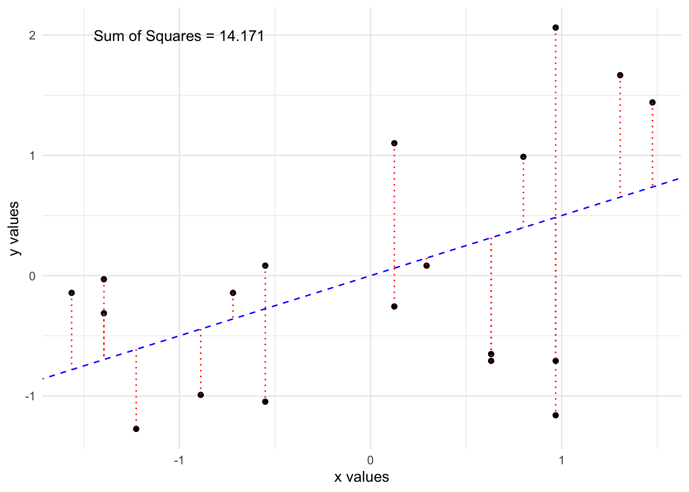
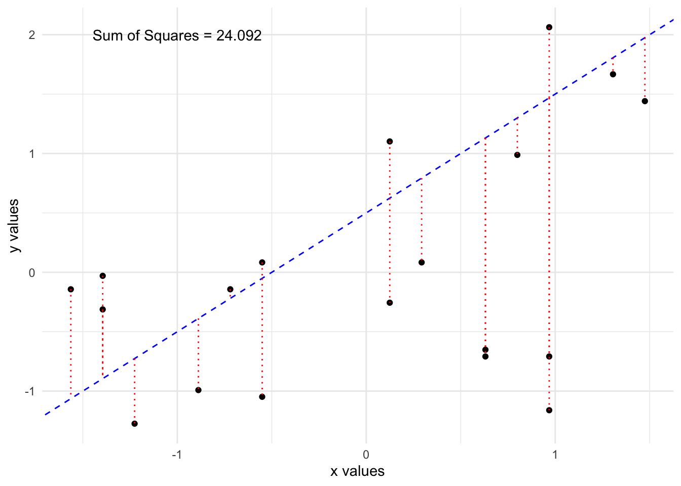
By eye, the first line looks to fit the data better and we see it has a lower sum of squared residuals. It turns out, there is a formula which will give us the “best” line, which will minimize this quantity as much as possible.
Least Squares
Using Calculus, we can derive formulas for the optimal slope and intercept, \(\hat{\beta}_0, \hat{\beta}_1\), which minimize this squared sum of residuals.
These formulas are given by
\[ \hat{\beta}_0 = \bar{y} - \hat{\beta}_1 \bar{x} \]
\[ \hat{\beta}_1 = corr_{x,y}\frac{s_y}{s_x}, \]
where \(s_y\) is the sample standard deviation of \(y\), \(s_x\) is the sample standard deviation of \(x\) and \(corr_{x,y}\) is the sample correlation between \(x\) and \(y\). These formulas don’t need to be mesmerized, but the interpretation, which we will see below, is very important.
We can also estimate the standard error of the residuals, i.e, how spread out they are. This is given by
\[ \hat{\sigma}_{e} = \sqrt{\frac{1}{n-2}\sum_{i=1}^{n}(y_i -\hat{y}_i)^2}, \] where we use \(n-2\) because we have to estimate two parameters, \(\hat{\beta}_0\) and \(\hat{\beta}_1\). This is known as the standard error of the regression.
Example
If we wanted to fit a regression to the penguin data then \(x\) is the flipper length and \(y\) is the body mass.
For this we can get the coefficients using the sample means and standard deviations \(\bar{x}=\) 200.915, \(\bar{y}=\) 4201.754, \(s_x=\) 14.062, \(s_y=\) 801.955, and \(corr_{x,y}=\) 0.871.
We can plug these numbers in to get
\[ \hat{\beta}_1 = 0.871 \frac{801.955}{14.062} = 49.67 \]
\[ \hat{\beta}_0 = 4201.754 - 49.67 \times 200.915 = -5777.694 \]
2.3 Conditions for Linear Regression
A linear model is likely at best an approximation to our real data and so we must examine the validity of the approximation. Many of the conditions can be investigated by looking at the residuals of the model (the distances we saw above).
Generally, we require 4 conditions to be true before fitting linear regression:
There is some linear trend in the data, not some non linearity.
The residuals \(e_1,e_2,\ldots,e_n\) are independent. That means that there is no obvious pattern in the residuals, such as many positive values in a row. We want our underlying pairs (\(x_i,y_i\)) to be independent of each other, just like we wanted our data to be independent when doing tests in the previous section.
The residuals are approximately normally distributed with mean 0. We run into problems if there are some residuals very far from 0.
The variance of the residuals should not change as \(x\) changes.
We want to keep these conditions in mind every time we fit a regression.
Properties of these estimators
After fitting this regression we can show that:
\(\sum_{i=1}^{n}e_i = 0\), the sum of the fitted residuals when the model includes an intercept term. This is always true, and does not mean that a linear model is correct.
The regression line will go through the point \((\bar{x},\bar{y})\), if there is an intercept term. This is also always true and doesn’t mean the model is correct.
Checking Conditions
We do need to investigate the other assumptions for fitting a linear regression. There are several ways to do this. Let’s first look at the fitted regression model for the penguin data and check whether the assumptions look reasonable.
For every point we can compute its residual by calculating the vertical distance from the point to the line,
\[ e_i = y_i -\hat{y}_i, \]
we will then examine these residuals and see if the assumptions we made are reasonable. We will do this in several ways.
Histogram of Residuals
Our model assumes that the residuals are approximately normal with mean 0. If this is true, a histogram of the residuals should look like it came from that distribution. It particular, it should be centered near 0, and have a similar spread on both sides. We should not see patterns such as many more negative residuals than positive residuals.
This condition can often be satisfied even when a linear model is not correct, so residuals which look to be normally distributed about 0 is only a small piece of checking whether the model is sensible.

Residuals against fitted values
A second check is to plot the fitted values (\(\hat{y}\)) against the residuals \(e_i\). This lets us check if the residuals are independent of the fitted values and if the variance of the residuals changes as we change \(x\) (which would change as we change \(\hat{y}\)).
Lets do this plot for this example.
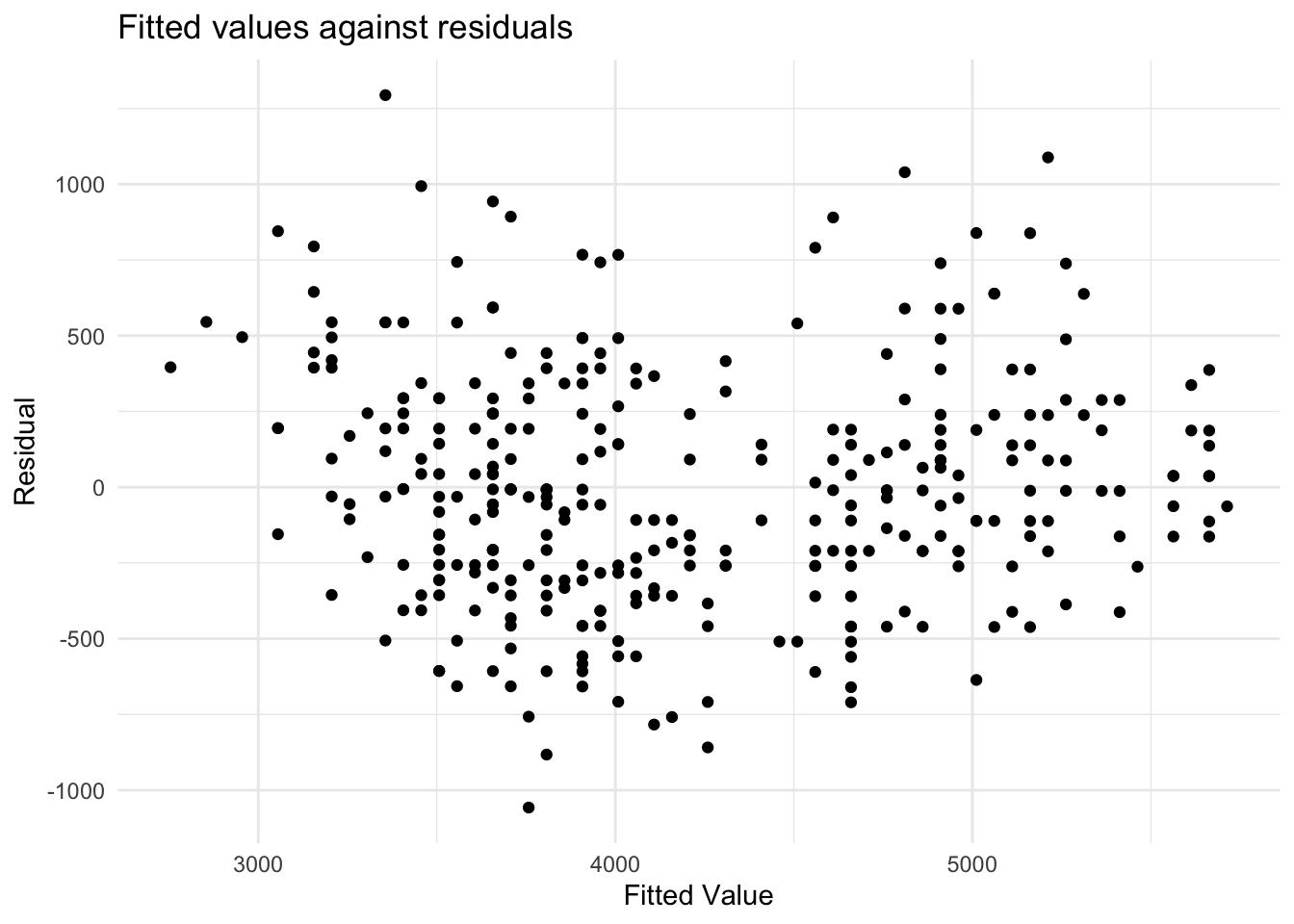
Here we are checking two things:
- Are the residuals independent of the fitted value? There are a similar number of positive and negative residuals and they seems to be spread across the range of fitted values. Also, the largest positive value is about as far from 0 as the smallest negative value. Based on this plot, it does appear that the residuals are independent of the fitted value.
- Does the variance of the residuals look similar as we change the fitted value? That is, if we took some values of \(x\), is the spread of the \(y\) values similar at these values? This looks to be true here. So, based on what we have checked so far, we have no reason to think our regression model is not appropriate. This means, if we interpret our regression model, which we will cover shortly, the interpretation will be reasonable.
Normal Plots
One challenge you may have noticed with the above plots is that we are just judging by eye whether our data looks reasonable. We might also want a plot where we are checking whether the data shows a very definite pattern or not. A normal quantile plot gives us this.
It orders and plots the residuals against how we would expect them to look if they were independently drawn from a normal distribution. This true model would correspond to them being along the line shown.
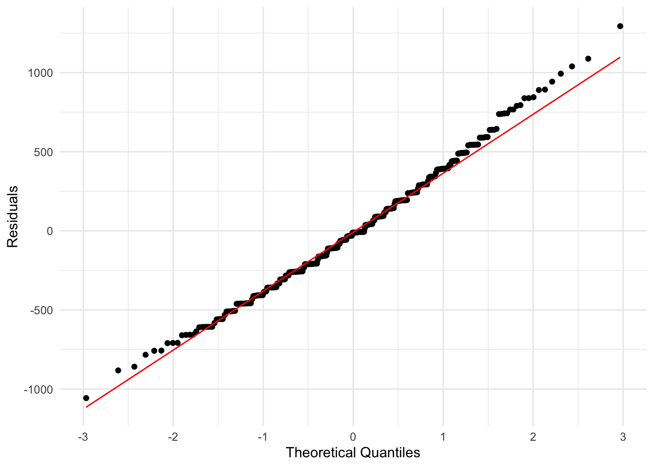
Here we do not have points which widely differ from the line, so again this suggests that our regression model is a reasonable way to model this data.
We will next see that the problems with a model can be much more obvious.
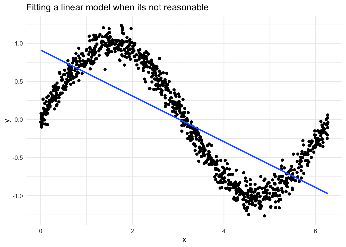
When things are very wrong
Here is an example where the data is clearly not linear at all. Thankfully, from looking at the residuals, we can see clearly that the assumptions are violated.

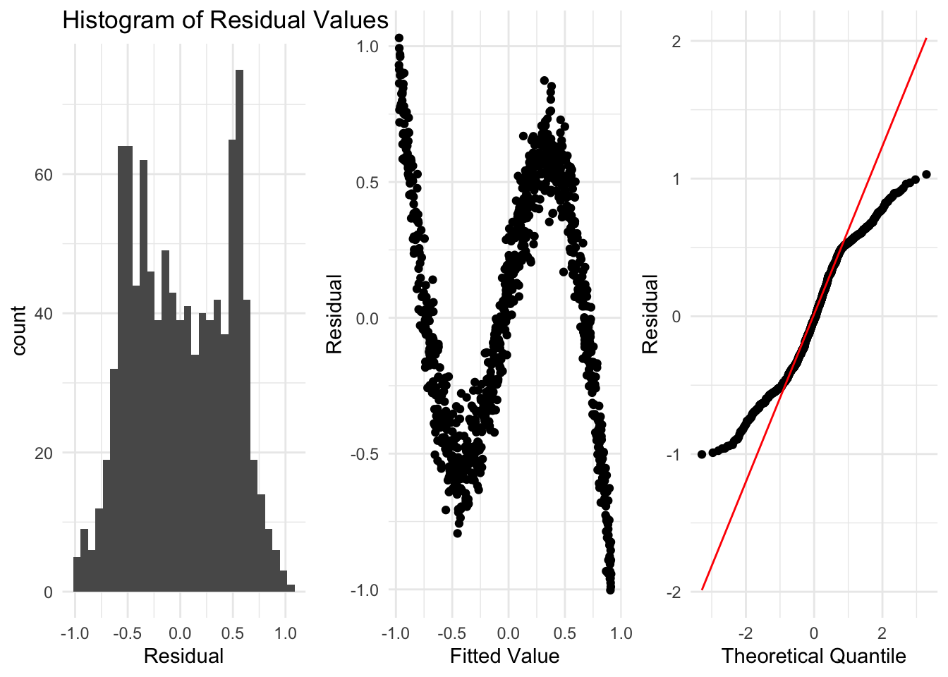
Here we see things in each of the residual plots that indicate we have a problem, and that a linear regression is not suitable for this data.
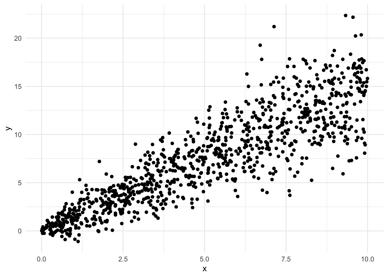
Another Bad Example
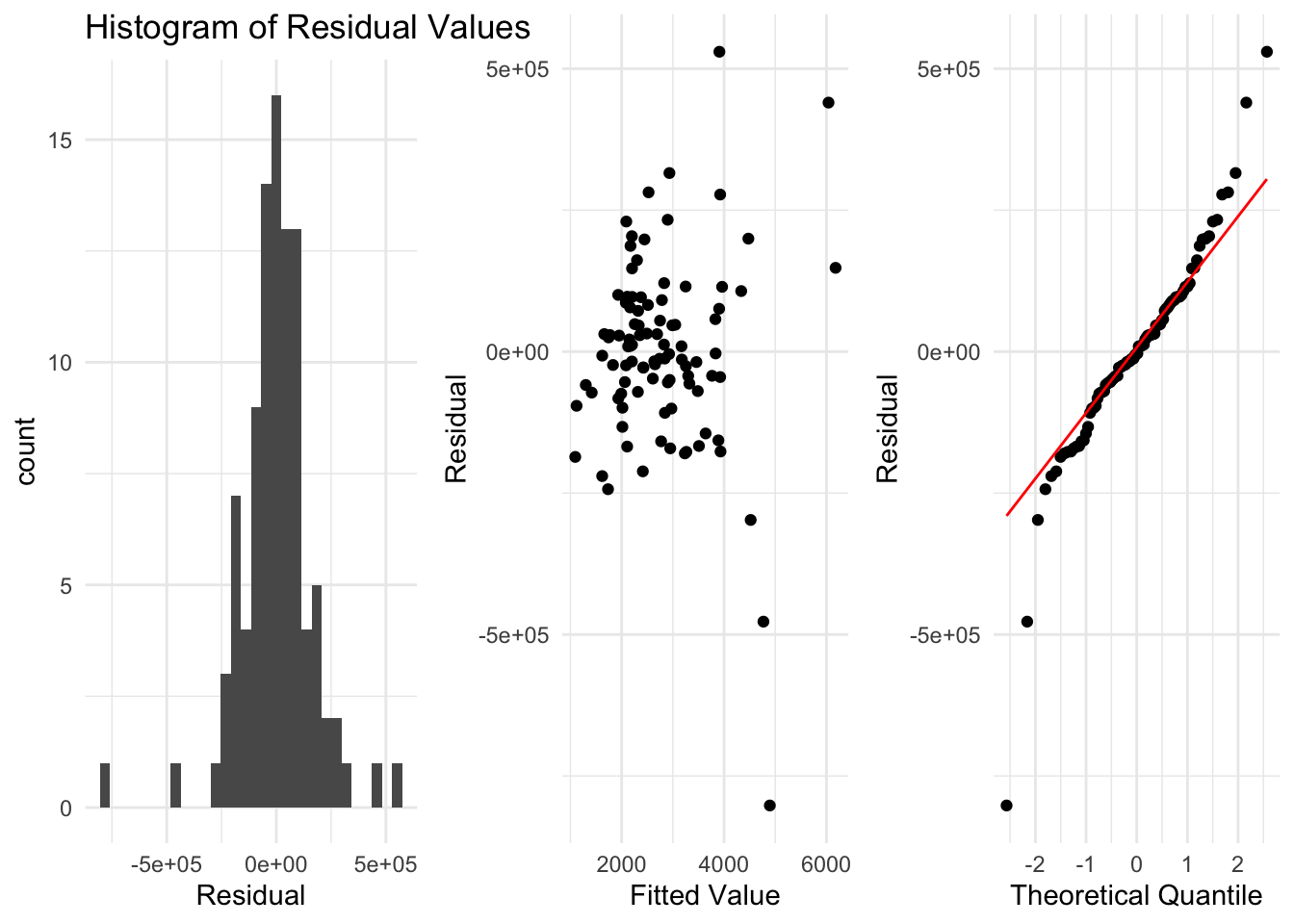
Here is an example where at first a linear regression might look quite reasonable. However, when we look at the residuals, we see some clear violations of the assumptions. These indicate a linear regression is not suitable for this data. Although the data is generally linear, because it doesn’t satisfy the other conditions a linear regression model is not appropriate.
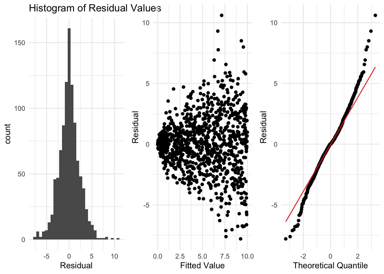
In this example, the histogram of the residuals looks good, and the data looks to be centered around 0. However, when we plot the residuals against the fitted values, we see some issues. As the fitted value increases, the residuals spread out much more. This indicates that the variance of the residuals changes as the fitted value changes. Similarly, in the normal quantile plot we see that at either end of the line points are very far from the line. This is a clear violation of the assumptions of a linear regression model. The variance of the \(y\) variable changing as \(x\) changes is known as heteroscedasticity.
Summary so far
So far we’ve seen how to fit a regression using the formula for the intercept and slope parameters. We can always fit a regression to data, but before we go any further we need to look at the residuals from the fitted model and see if they agree with the assumptions of a regression model. If we can see no patterns in the residuals and they look like random noise (samples from a normal distribution), then we can continue and begin to interpret what the regression tells us about the data. If we look at the residuals and conclude there is patterns in them which make them look non random, then we should conclude that a linear regression is not correct for that data. There may be something else we can do, or we may just need another model (possibly not covered in this class).
Another Example
Before moving on, lets first check one further example for the possible problems we could have. Lets look at the relationship the area of a house and its price for data collected in North Carolina. From an initial plot of the data, it seems like maybe we can say there is a linear relationship between the size of a house and its price. We first fit a regression and check the residuals before we can interpret the model.
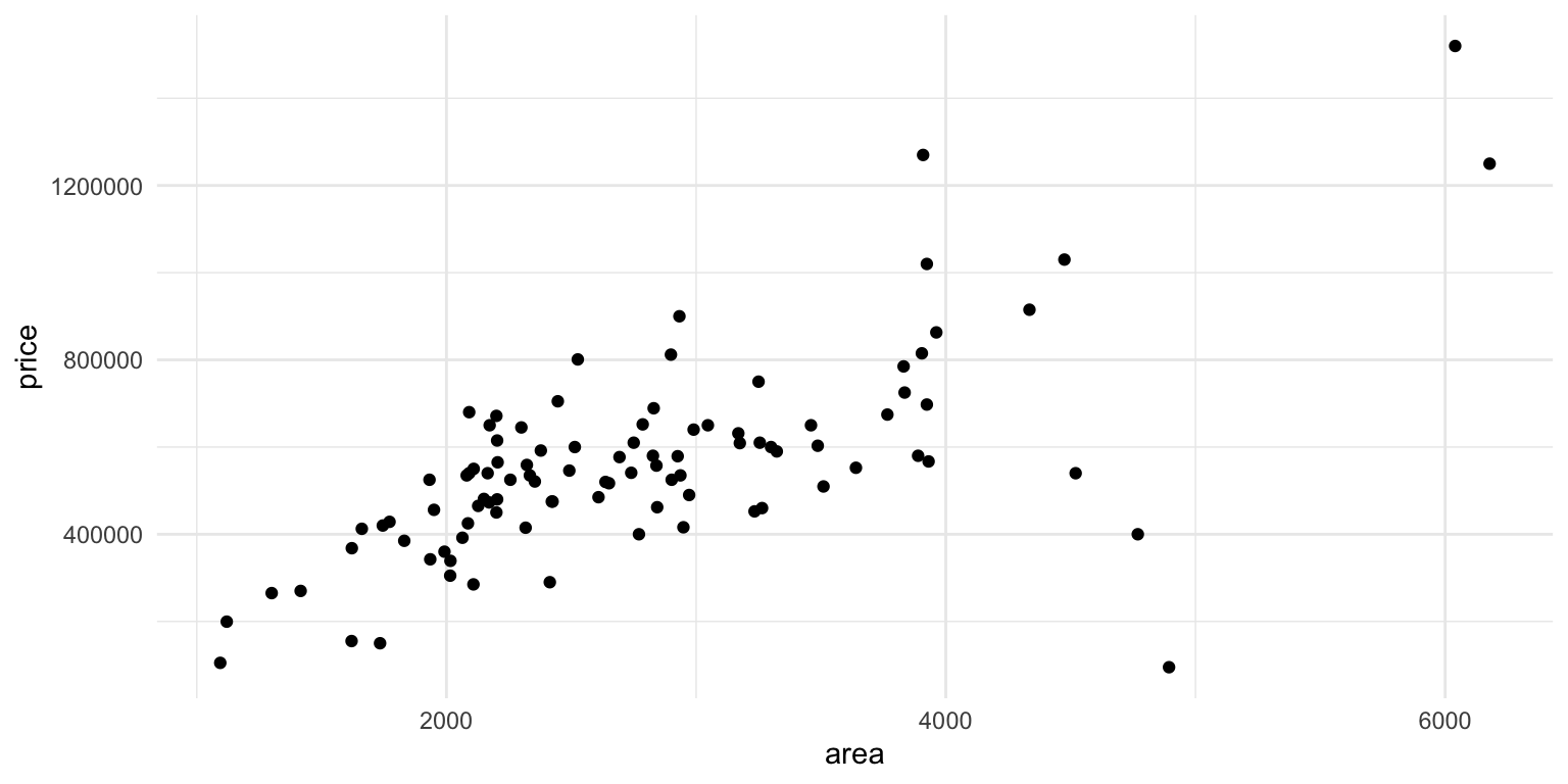
However, when we examine the residuals using the plots we described above, we see some issues that indicate our model might not be ok. It does appear that when the fitted value is larger the residuals are more spread out. We also see this in the quantile plot, where at either end we get points far from the line.
So, from what we know so far, we cannot use a linear regression for this data. However, we may be able to find ways to improve this later.
2.4 Interpreting a Regression Model
The coefficients
If we have determined a regression is appropriate for our data, then the estimated coefficients, \(\hat{\beta}_0,\hat{\beta}_1\) can be used to describe the relationship in the data.
The slope coefficient \(\hat{\beta}_1\) gives the change in the average value of \(y\) as we increase the \(x\) value by one unit.
Similarly, the intercept term \(\hat{\beta}_0\) gives the expected average value of \(y\) when \(x=0\), if the model is reasonable there (will see more next).
Example
For the penguin example we get
\[ \hat{\beta}_0 = -5780, \hspace{1.5cm} \hat{\beta}_1 = 49.686. \]
The intercept term not really interpretable, as it doesn’t make sense to have a flipper with 0 length.
\(\hat{\beta}_1=49.686\) means that as we increase the flipper length by 1mm, we expect the weight of penguins to increase by 49.69 grams, on average.
We can also use the regression coefficient estimates to get the expected mean value of the \(y\) variable at a specific \(x\) value.
The linear regression model says the expected (average) value of \(y\) for a given \(x\) is given by \[ \mathrm{Expected}(y) = \hat{\beta}_0 + \hat{\beta}_1 x \]
Using our linear regression fit, the expected body mass for a penguin with flipper length 200mm is \(-5780 + 49.69(200) = 4157.1\) grams. This corresponds to the y coordinate of the fitted line when \(x=200\).
Fitted Regression Line
R-Squared
Even if, after looking at the residuals and concluding a linear regression is reasonable, that might not mean a linear regression can describe the relationship between the variables well. We want to be able to quantify this somehow, using a number.
Before we said that the formula for the slope, \(\beta_1\), can be written in terms of the sample correlation \(corr_{x,y}\).
The square of this, written as \(R^2\), is widely used to describe the strength of a linear fit.
This is a number between 0 and 1, where larger values indicate a stronger relationship.
\(R^2\) describes how much variation there is about the fitted line, relative to the total variance of the \(y\) variable.
If we fit the model and compute the residuals \(e_1,\ldots,e_n\) then with \(s^2_{e}\) the squared error of the residuals \(s^2_{e}=\sum_{i=1}^{n}(y_i-\hat{y}_i)^2\), and \(s^2_{y}\) the squared error in \(y\), \(s^2_{y}=\sum_{i=1}^{n}(y_i -\bar{y})^2\), we can write
\[ R^2 = \frac{s^2_y - s^2_{e}}{s^2_{y}}. \]
This describes how much of the the variability of \(y\) is captured by the regression model.
As the variance of the residuals decreases, this number will be closer to 1.
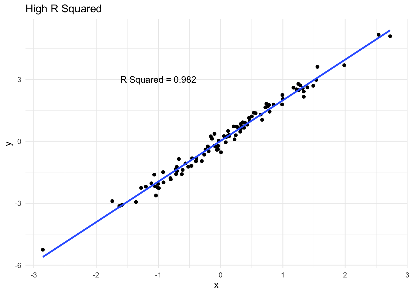
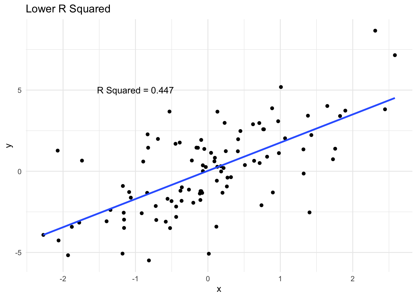
How R Squared varies
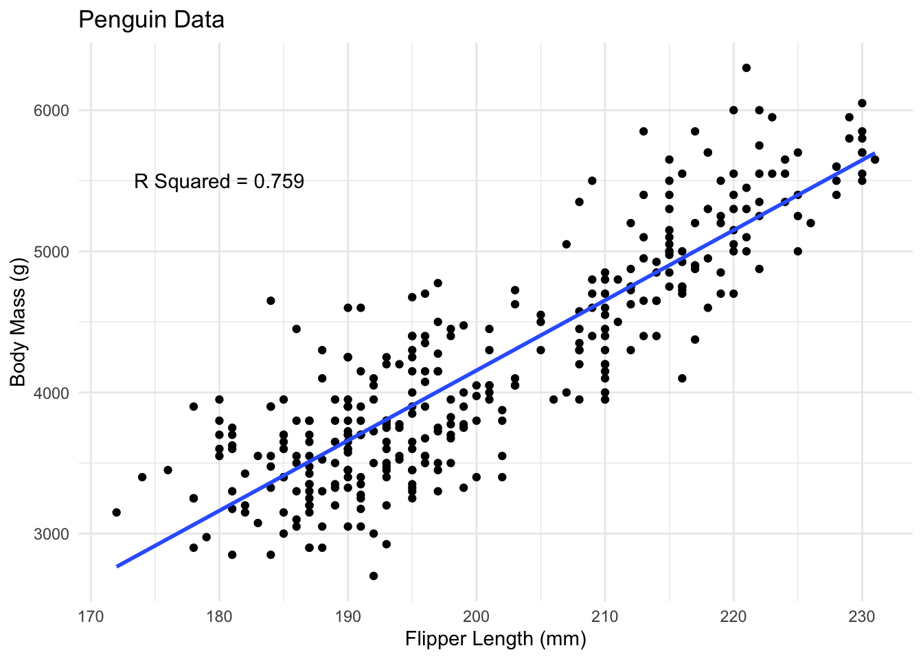
We can see a few examples of how closely data follows a line and the corresponding \(R^2\). A high \(R^2\) means that the variability in \(y\) is largely captured by the line.

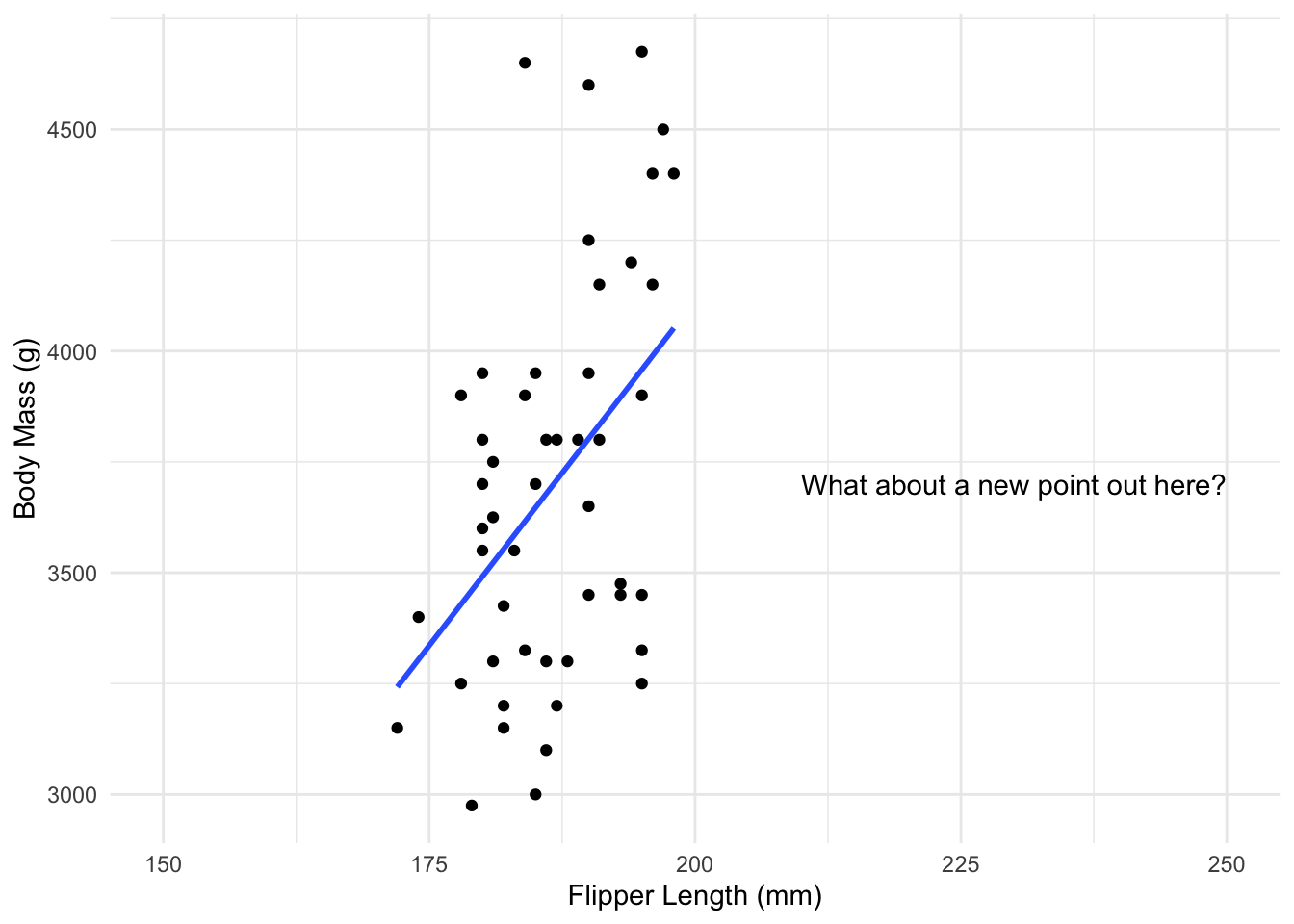
Dangers of extrapolation
While linear regression can work very well, it is somewhat dependent on the data you have, in many ways.
We saw that looking at the residuals of the model can help us figure out if a linear regression is reasonable for the data we have. This tells you a linear model is reasonable in the range of values of initial data. But in general there is no reason to think its also valid as we move far away from those points.
Some software helps with this, for example by not extending the line beyond where the data is.
2.5 Fitting a Regression in R
Fitting a linear regression is straightforward in most software packages, and is one of the mostly useful statistical tools. As important is being able to understand the output from fitting a regression model. This includes interpreting the estimates of the parameters, the estimate of \(R^2\) and other output.
Penguin Data
Lets fit the regression for the penguin data. To do this we will use the lm function. Here if we want to regress \(Y\) against \(X\) then the notation is lm(Y ~ X). If we have both these variables in a data frame, then we just need to write the variable names and specify the data frame they are in.
This creates an object which stores lots of information about the regression fit. We can see this by using summary.
penguin_fit <- lm(body_mass_g ~ flipper_length_mm,
                  data = penguins)

penguin_fit
We can see most of the important information by using summary.
# make sure this is wide enough to see all the output
summary(penguin_fit)
Call:
lm(formula = body_mass_g ~ flipper_length_mm, data = penguins)

Residuals:
     Min       1Q   Median       3Q      Max
-1058.80  -259.27   -26.88   247.33  1288.69

Coefficients:
                   Estimate Std. Error t value Pr(>|t|)
(Intercept)       -5780.831    305.815  -18.90   <2e-16 ***
flipper_length_mm    49.686      1.518   32.72   <2e-16 ***
---
Signif. codes:  0 '***' 0.001 '**' 0.01 '*' 0.05 '.' 0.1 ' ' 1

Residual standard error: 394.3 on 340 degrees of freedom
  (2 observations deleted due to missingness)
Multiple R-squared:  0.759, Adjusted R-squared:  0.7583
F-statistic:  1071 on 1 and 340 DF,  p-value: < 2.2e-16
This gives us different pieces of output:
Some summary statistics of the spread of the residuals.
The estimated slope and intercept, along with their corresponding standard errors, a t-statistic and the corresponding p-value.
The standard error of the residuals.
Two different versions of the \(R^2\)
An F-statistic and a corresponding p-value.
We will come back to most of these quantities. For now, we are only interested in the residuals, the estimated slope and intercept and the estimate of \(R^2\). The term Multiple R-squared is the one we discussed previously. The other is just a slight correction, which we will not discuss.
The residuals just show some quick properties of the model. Remember we want the spread of our residuals to be even about zero. This shows that the biggest positive and negative residuals are about as far from 0.
The estimated intercept and slope are just computed using the formula we discussed before. We will later use the standard errors to test whether these parameters are different from 0.
If you are just interested in the coefficients the function tidy in the broom package (which needs to be installed and loaded) gives a cleaner summary. We can also extract just the \(R^2\) on its own, which does not need the broom package.
tidy_coefs <- tidy(penguin_fit)
tidy_coefs
# A tibble: 2 × 5
term estimate std.error statistic p.value
<chr> <dbl> <dbl> <dbl> <dbl>
1 (Intercept) -5781. 306. -18.9 5.59e- 55
2 flipper_length_mm 49.7 1.52 32.7 4.37e-107summary(penguin_fit)$r.squared[1] 0.7589925Finally, we can plot the data points with the fitted regression line, using the function abline, where we pass in the regression fit directly.
Looking at the residuals
It is quite easy to do the residual diagnostic plots we saw above. When we fit a linear regression the residuals are saved. Above, we stored out fit in penguin_fit. We can then access the residuals using penguin_fit$residuals, which we can then use to look at a histogram of the residuals.
hist(penguin_fit$residuals)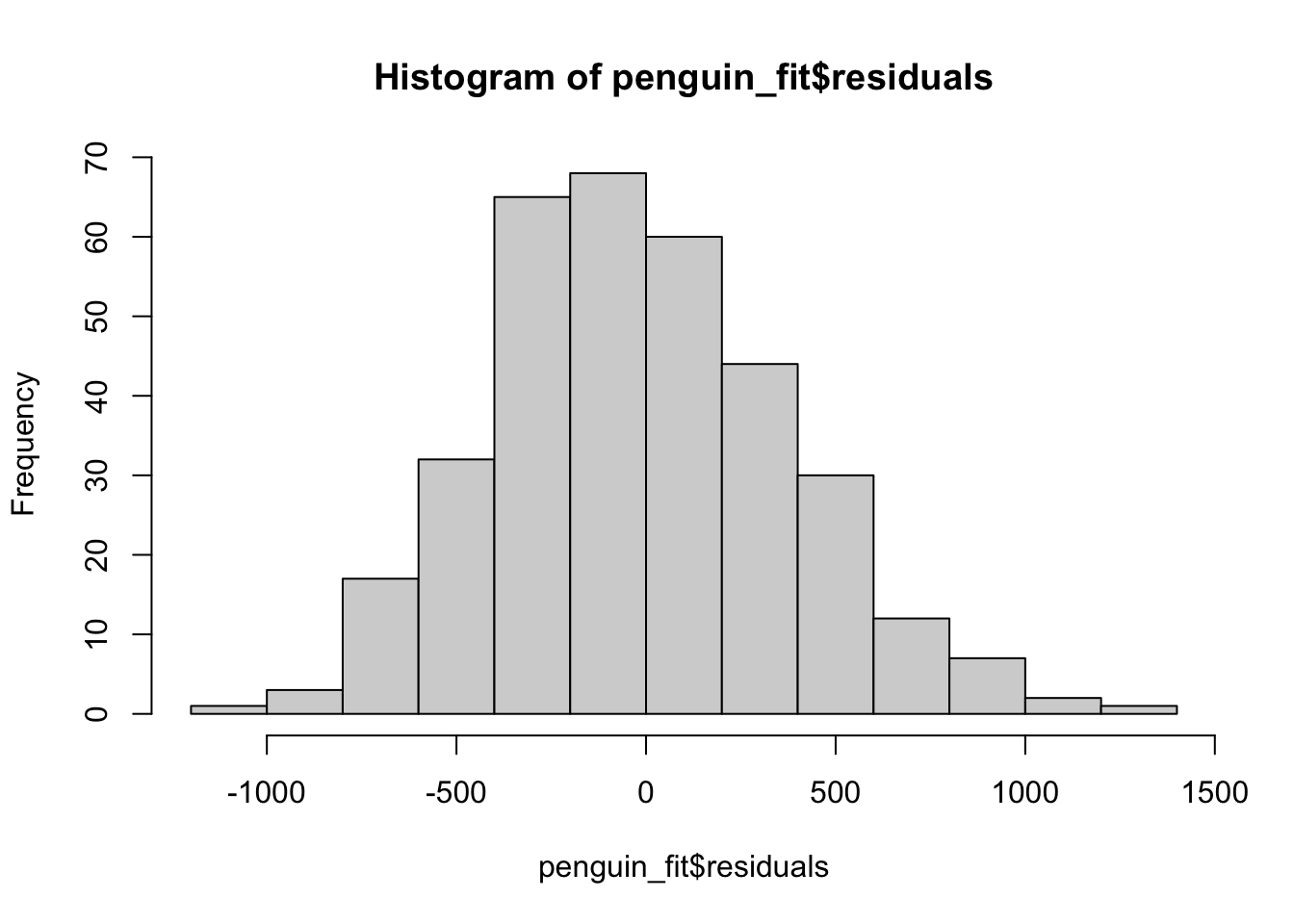
If we want to plot the fitted values against the residuals, the fitted values are also stored in penguin_fit$fitted.values. So we can do a scatter plot of these.
plot(penguin_fit$fitted.values, penguin_fit$residuals,
     main = "Residuals appear to satisfy assumptions")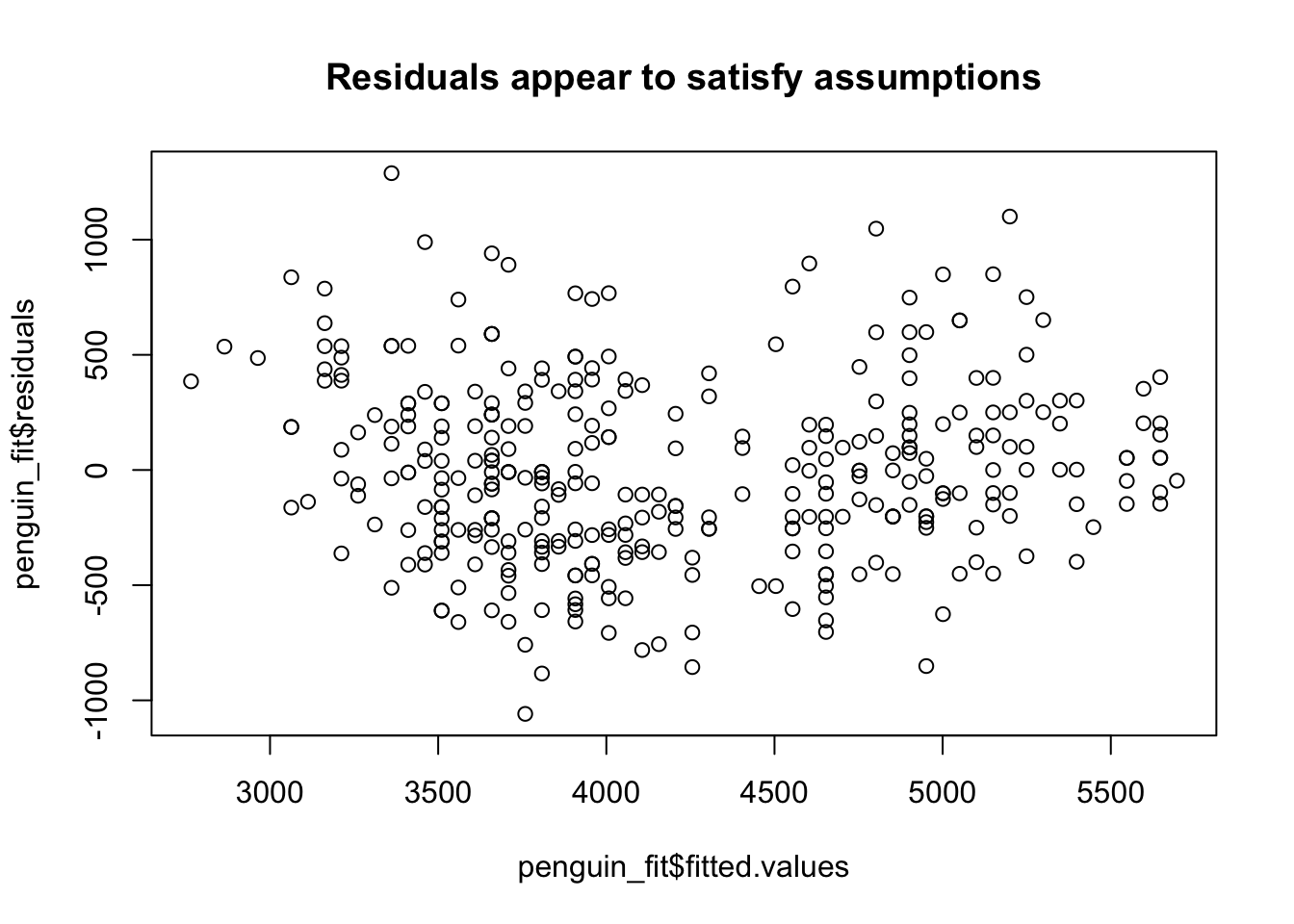
Similarly, if we wish to do a normal probability plot, we use the function qqnorm, passing in the residuals. We then add the diagonal line to the plot using qqline. These need to be run together to correctly add the line.
qqnorm(penguin_fit$residuals)
qqline(penguin_fit$residuals, col = "Red")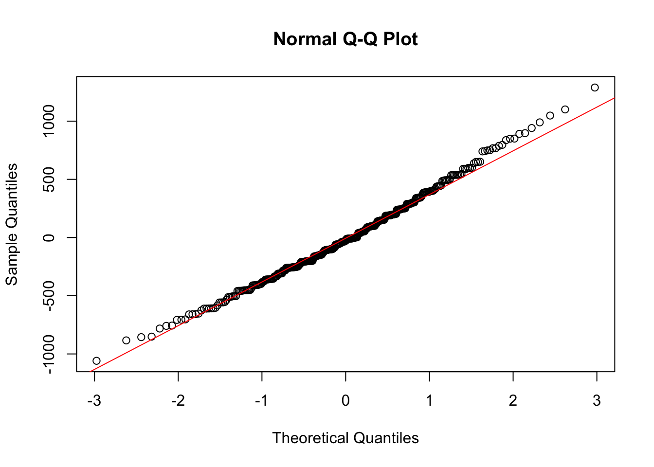
2.6 Transforming Data
We’ve see that linear regression can work very well, but for some data it just isn’t that suitable. Much of the time, this can’t be avoided and another method needs to be considered, such as some of the methods we will see later.
However sometimes, we can actually reexpress the data in such a way that a linear regression is then appropriate. This can lead to a scenario where we can fit a good linear regression. We can then use this regression to get information about the scale of the data we were interested in.
As a very simple example, consider the following data, which looks at the relationship between the volume and diameter of cherry trees.
url <- "https://www.openintro.org/data/csv/cherry.csv"

tree_data <- read.csv(url)

lm(volume ~ diam, data = tree_data)
Call:
lm(formula = volume ~ diam, data = tree_data)

Coefficients:
(Intercept)         diam
-36.943 5.066 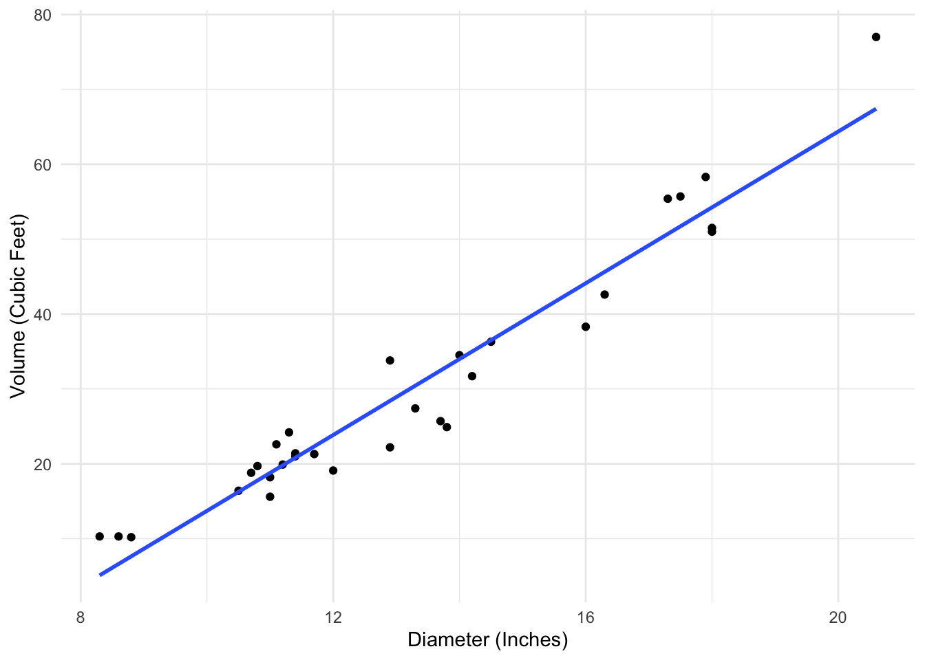
If we convert these measurements to centimeters and cubic meters, our estimated regression will change but it won’t really change our understanding of the data. It will just change the \(x\) and \(y\) axes on the plot.
metric_data <- tree_data %>%
  mutate(metric_vol = volume/35.315,
         metric_diam = diam * 2.54)

lm(metric_vol ~ metric_diam, data = metric_data)
Call:
lm(formula = metric_vol ~ metric_diam, data = metric_data)

Coefficients:
(Intercept)  metric_diam
-1.04611 0.05648 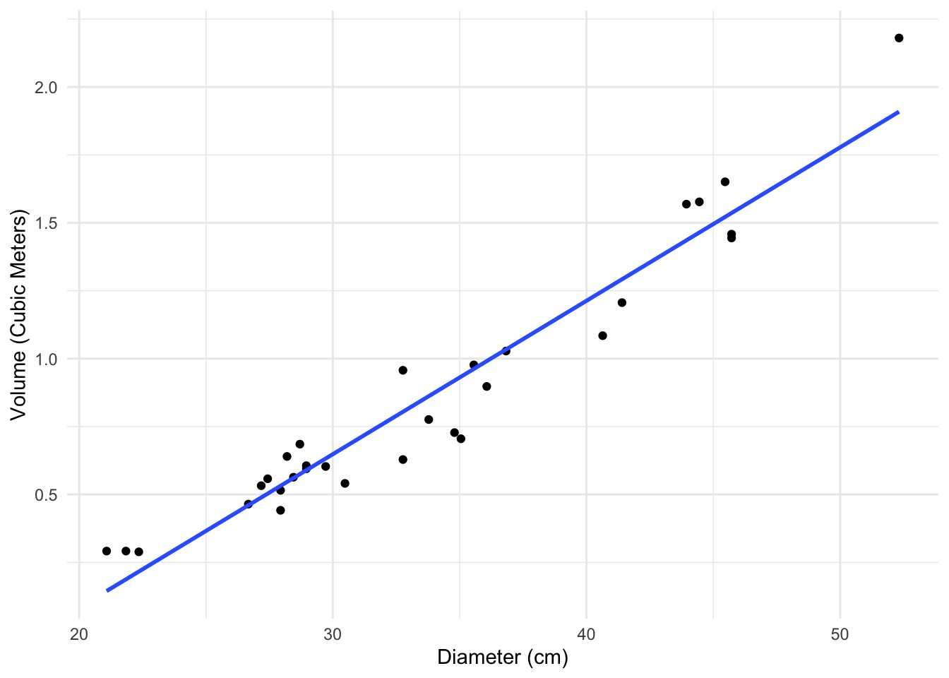
The transformations we will see below don’t really change the data either, they just express it in a different way.
Rescaling the Y variable
Lets look at an example where we have a wide range of values of both \(x\) and \(y\), looking at the number of species on islands with different land area.
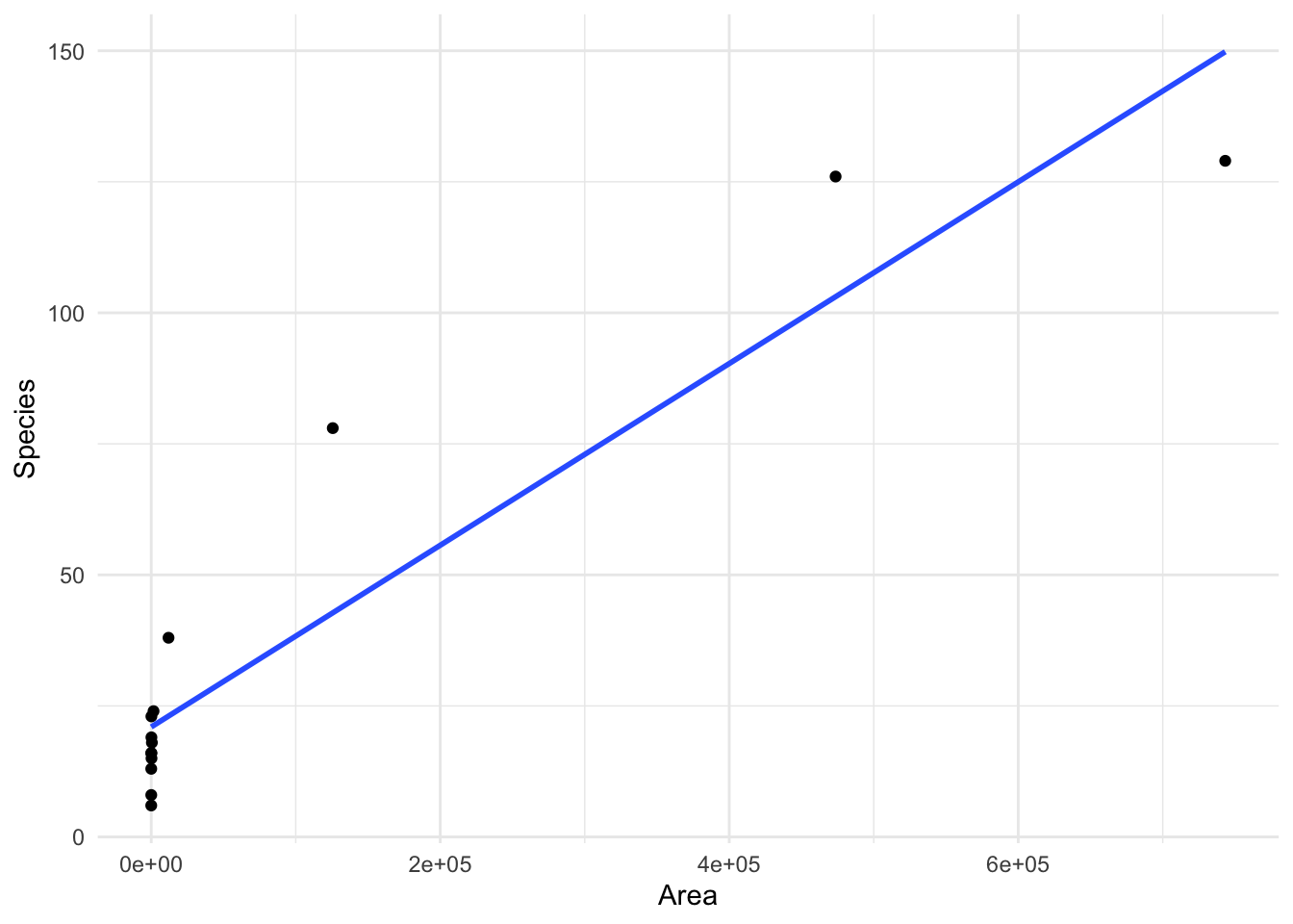
We can see that when we fit a linear regression we do not perform particularly well, and there appears to be some patterns present in the residuals which we would like to remove.
island_fit <- lm(Species ~ Area, data = species_data)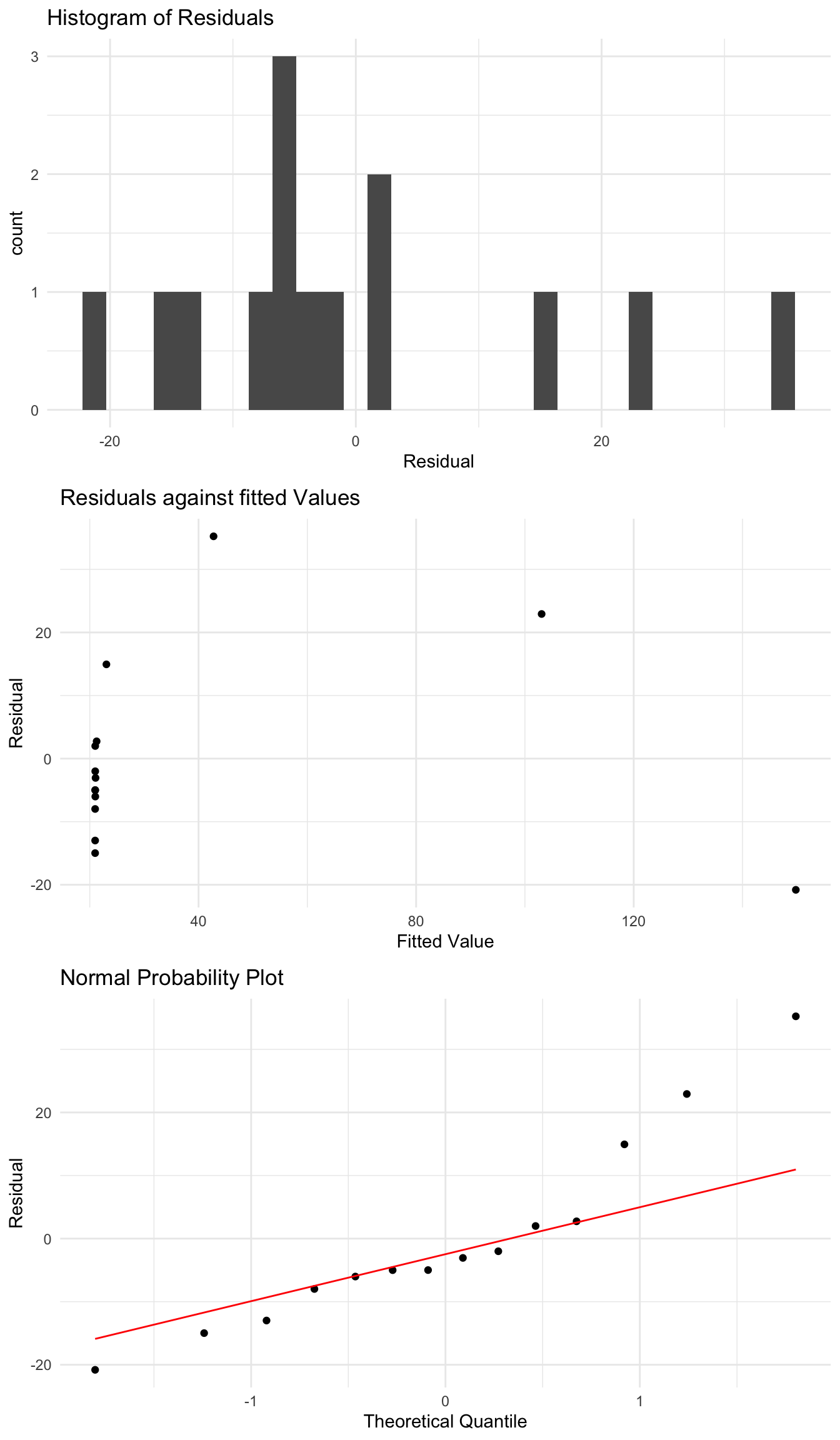
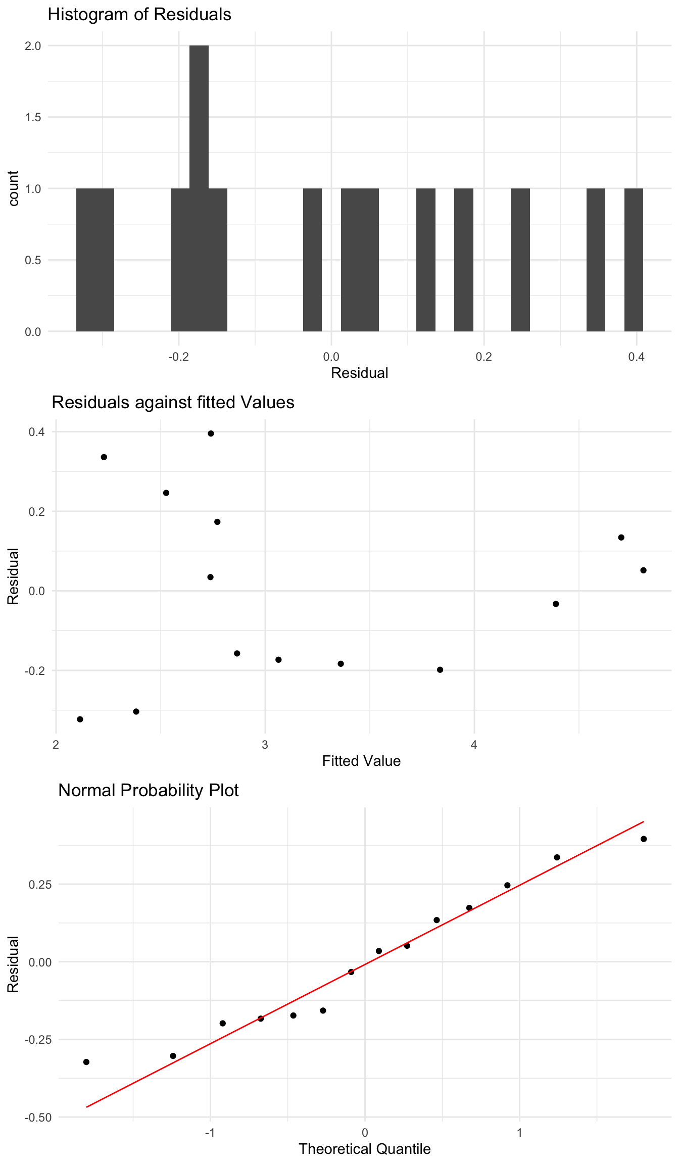
When we look at the residuals of this model using the plots we saw before, we see that there are some problems and clear patterns in the residuals as the \(x\) variable changes. Lets instead try regressing \(X\) against \(\log(Y)\), which gives the model
\[ \log(Y) = \beta_0 + \beta_1 X + \epsilon \]
It is straightforward to also fit this model in R, with just a small change. Then we can look at the residuals of this modified model instead
log_fit <- lm(log(Species) ~ Area, data = species_data)
log_fit
Call:
lm(formula = log(Species) ~ Area, data = species_data)

Coefficients:
(Intercept)         Area
2.860e+00 3.305e-06 
These residuals seem to be slightly more reasonable than the original version. One reason to do a transformation is that we have a very large range of values of the \(y\) variable possible here.
We can also consider other transformations of \(y\), with the next common one being
\[ \sqrt{Y} = \beta_0 + \beta_1 X + \epsilon. \]
Again, we can easily fit this model in R. We can look at the residuals under this model also.
sqrt_fit <- lm(sqrt(Species) ~ Area, data = species_data)
sqrt_fit
Call:
lm(formula = sqrt(Species) ~ Area, data = species_data)

Coefficients:
(Intercept)         Area
4.370e+00 1.138e-05 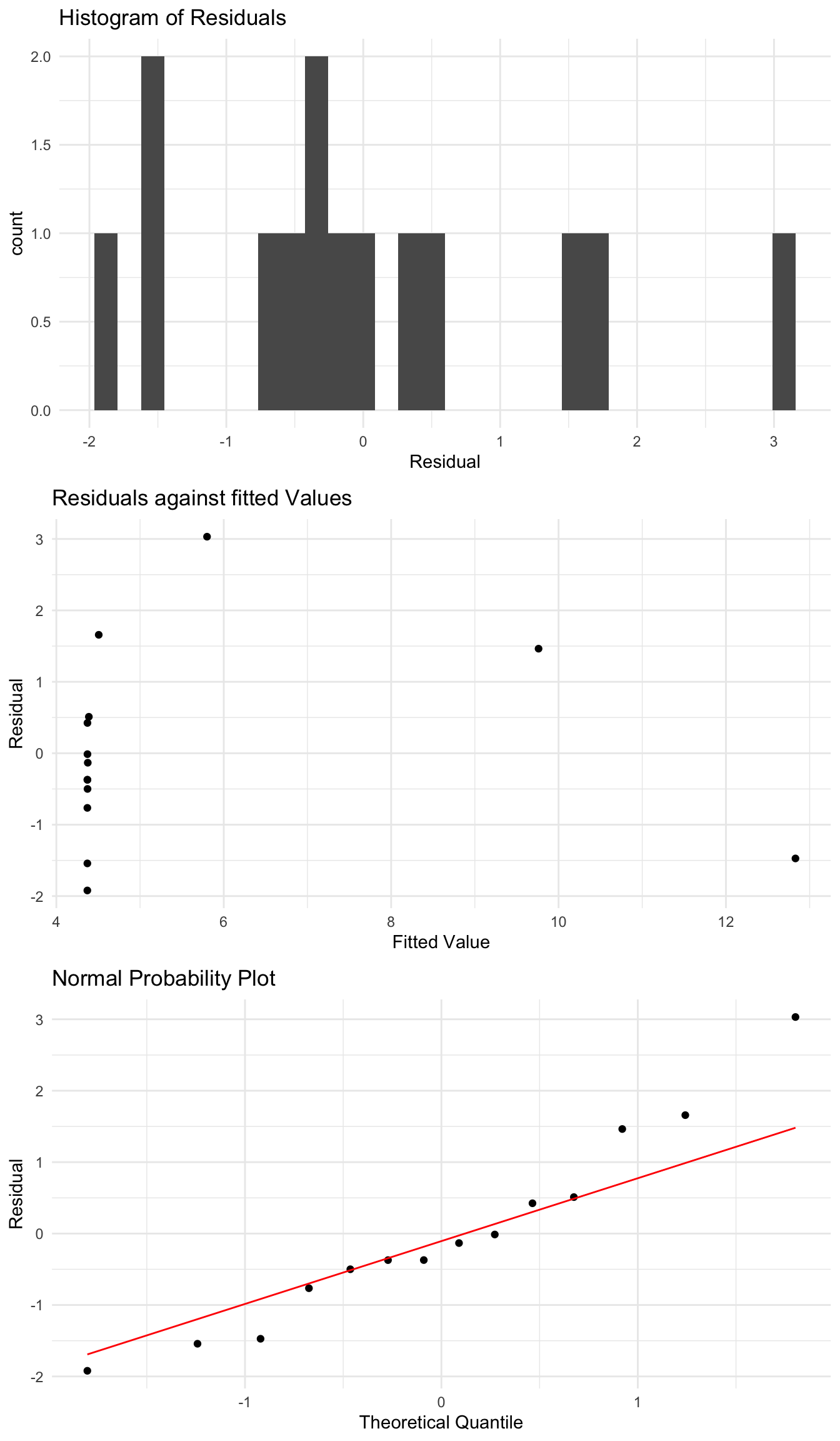
Here we see an improvement in the plots. The quantile plot looks quite good, and the only concern would maybe be the second plot. But this is a good example of where this transformation definitely improves the regression. If we could also transform the \(X\) variable, which we will see below, we can likely construct a good model for this data. We can also do other transformations of \(Y\) such as \(1/Y\), which just require modifying \(Y\) inside the lm function.
Estimating after transformation
How do we interpret the results of these regressions on this new scale?
We said before that \(\hat{\beta}_1\) gives the change in the average value of \(y\) as we increase the \(x\) value by one unit.
If instead we have \(\log(y)\) then we can say that \(\hat{\beta}_1\) gives the change in the average value of \(\log(y)\) as we increase \(x\) by one unit.
Looking at the estimated coefficients for the log regression, we see the estimate of \(\hat{\beta}_0\) is 0
log_fit$coefficients (Intercept) Area
2.860173e+00 3.305286e-06 So this says that, on average, if the area of an island increases by 1 square km, the \(\log\) of the number of species is expected to increase by \(3.31\times10^{-6}\), on average. Note that the intercept term corresponds to the expected log number of species on an island with 0 area, so we don’t need to really consider this.
How do we interpret this transformed linear regression? After we fit the regression \[ \log(Y) = \beta_0 + \beta_1 X + \epsilon, \]
we get estimates \(\hat{\beta}_0,\hat{\beta}_1\). What do they mean now?
Estimate \(\hat{\beta}_0\) tells us the average value of \(\log(Y)\) when \(X\) is 0!
Similarly, \(\hat{\beta}_1\) tells us that as we increase \(X\) by one unit, we expect the log of Y to increase by \(\hat{\beta}_1\), on average
Similarly, for a specific value of \(X\), the model will give an estimated value for \(\log(Y)\) on the line of
\[ \log(Y) = \hat{\beta}_0 + \hat{\beta}_1 X. \]
We probably care more about the original \(Y\) variable. So to get that we can take the exponential of of both sides, getting
\[ Y = e^{\hat{\beta}_0}e^{\hat{\beta}_1 X}. \]
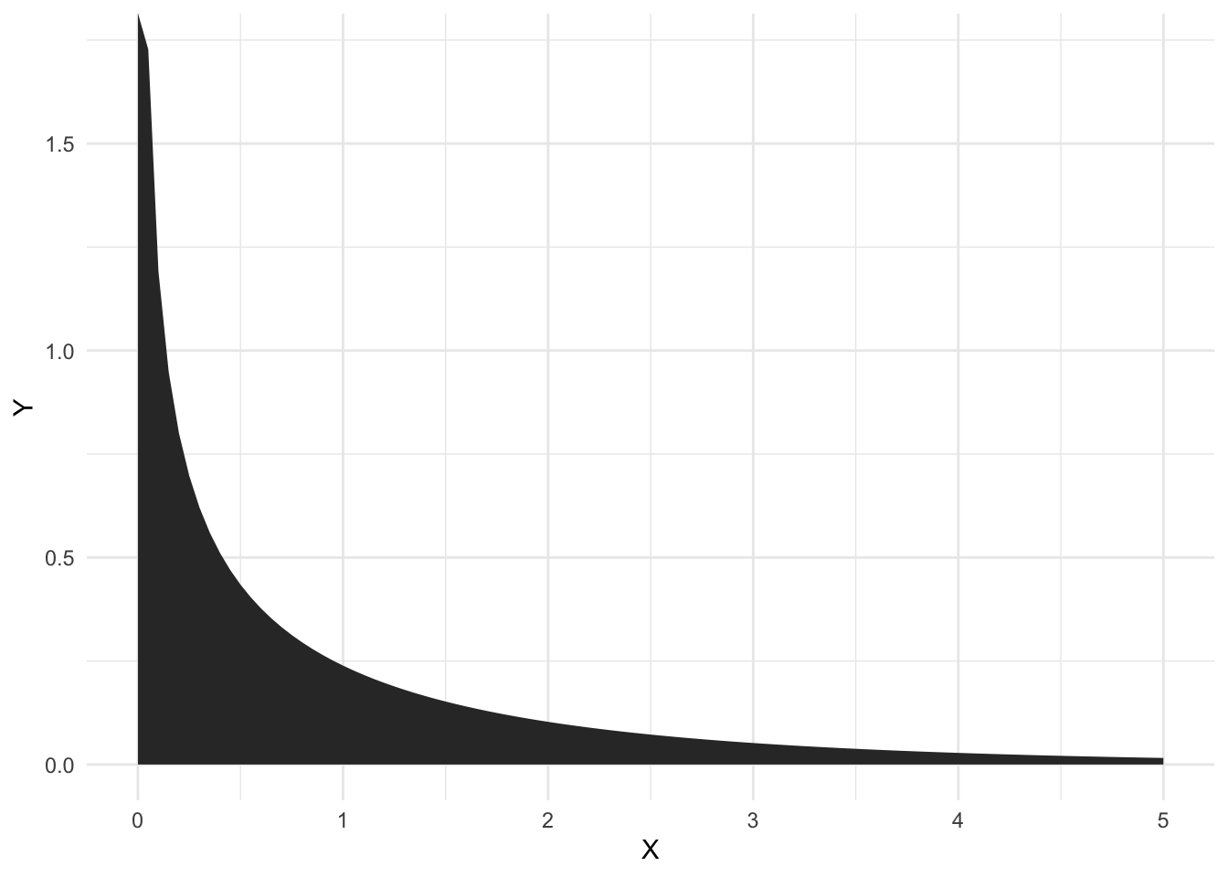
To show this, lets plot the regression “line” we get from this log transformation. When we show it on the original scale of \(Y\) it is not a line at all, but a curve.
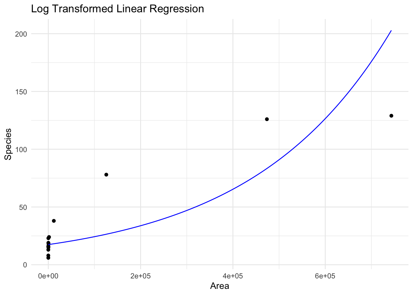
Another thing to note is that we will get different estimates from the regression if we use \(\log(Y)\) or not, for the same value of \(X\). For this example, lets see what the \(y\) value on the line is when Area=10000.
The original model, with no transformation, gives
giving an estimate
\[ \hat{y} = 20.98 + (1.733\times 10^{-4})\times(100000) = 38.31. \]
If we estimate for the same \(X\) under the log model, we instead have
Call:
lm(formula = log(Species) ~ Area, data = species_data)

Coefficients:
(Intercept)         Area
  2.860e+00    3.305e-06
giving an estimate
\[ \hat{y} = \exp(2.86 + (3.305\times 10^{-6})\times(100000)) = 24.31 \]
Similarly, if we instead want to look at the fitted value under the sqrt fit, we then have
\[ \sqrt{Y} = \beta_0 +\beta_1 X \]
so this gives
\[ \hat{Y} = (\hat{\beta}_0 + \hat{\beta}_1 X)^2. \]
So for this model the square root transformation instead gives
\[ \hat{y} = (4.37 + (1.138\times 10 ^{-5})\times (100000))^2 = 30.33. \]
If one transformation leads to residuals which look much better than the original data, then that might be appropriate to use. However, in practice, you are more likely to see a scenario like this, where the two transformations are an improvement over the original model but still not perfect. If you had to fit a model, either the log or sqrt is an improvement, but you might probably still have some concerns.
Transforming the X variable also
One way we can potentially improve this model further is by also transforming the \(X\) variable. In this example we saw that there is large variability in \(X\), with a small number of very large values. Applying a log transform to \(X\) could also impact the residuals.
The most common such model is to do a log transformation of both \(X\) and \(Y\), which can be done using the lm function also.
Call:
lm(formula = log(Species) ~ log(Area), data = species_data)

Coefficients:
(Intercept)    log(Area)
     1.6249       0.2355
Just like before, we can see what the residuals look like after this transformation, and if they look more reasonable.
Like before, it can be hard to say for certain if one such transformation is better than another.
Interpretation of log-log Regression
When we take the log of both \(X\) and \(Y\) we have
\[ \log(Y) = \beta_0 + \beta_1 \log(X), \]
so taking the exponent of both sides gives
\[ Y = e^{\beta_0}X^{\beta_1}. \]
So for our fitted model, this gives estimated species with area of 100000 square km of
\[ \hat{y} = \exp(1.63)100000^{0.2355} = 76.81. \]
When using a transformation to fit a linear regression, you need to be aware of how you interpret the output for the original \(Y\), which is the variable you care about.
2.7 Outliers and Influential Points
Sometimes we fit a regression to data and there is one point which is very different to the other data, and gives us a residual much larger than the rest of our points? Could this be an issue with our model? Could this single data point have an impact on the model we fit?
We will illustrate this using an example from Stat2.
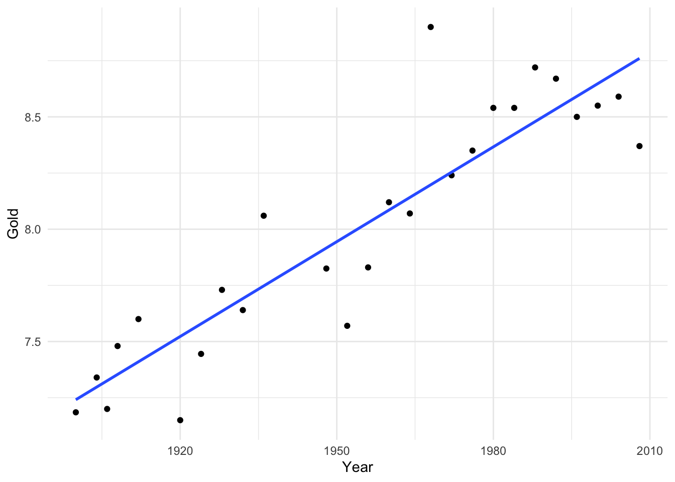
Here, when we fit a linear regression, most points lie quite close to the regression line. However, one point, the winning distance in 1968, is much further from the line than other points. This is even more obvious when we look at the residuals.
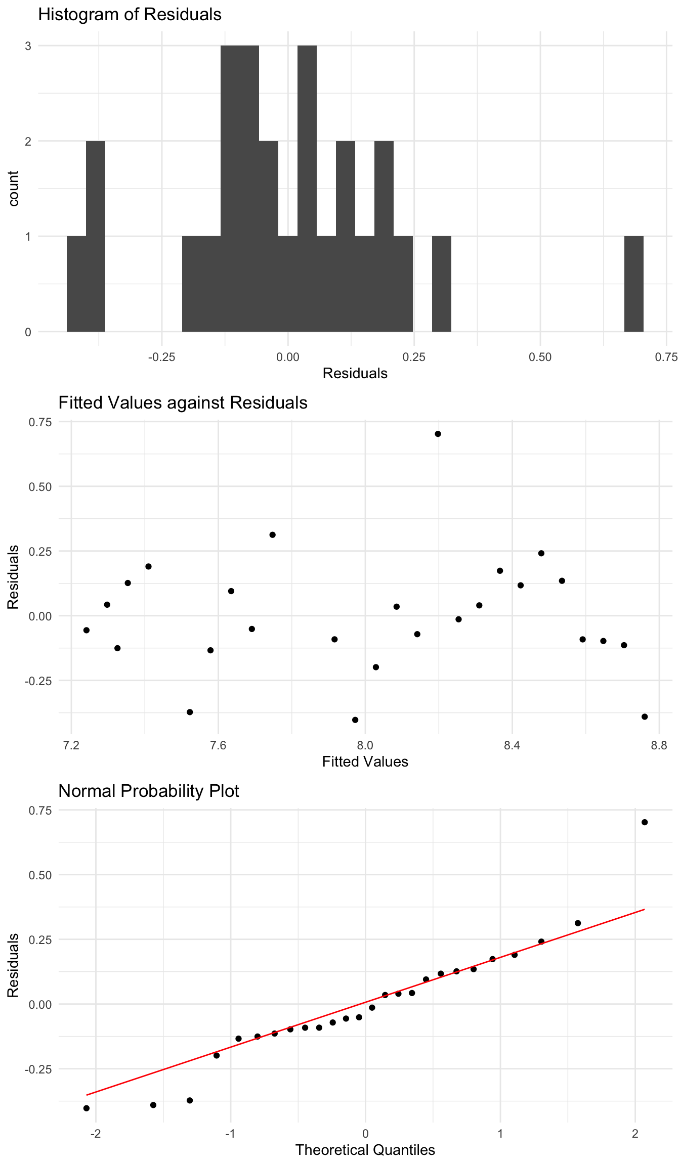
This single point has residuals which look unusual compared to the rest of the data. Do we need to deal with it?
We can compute standardized residuals also, which are given by
\[ \frac{y - \hat{y}}{\hat{\sigma}_e}. \]
This is just like computing z scores which we saw before. So values of a standarized residual larger than 2 would be unlikely and values larger than 3 or smaller than -3 would be quite unlikely.
How should we deal with points like this? The answer will really depend. For example, it could be the case that after identifying an unusual point like this, you can examine the original data and realise that someone simply wrote the number down wrong. But in general, unless there is some good reason to change or remove the point, it should probably be retained. In analysing data, it would be a good idea to highlight such unusual points, even if we cannot say any more.
In general, outliers should not be removed unless there is sufficient justification that that data point should not be in the same sample as the rest of the data.
Influential Points
It can also be the case that a single point can impact the regression you fit, and that removing a point would give a “better” model (if we can say better). For example, we can fit the above data, with and without the outlier point.
## load in the data
data_link <- "http://www.stat2.org/datasets/LongJumpOlympics.csv"
data <- read.csv(data_link)

## removing the unusual point
data_rm <- data[data$Year != 1968, ]

fit_rm <- lm(Gold ~ Year, data = data_rm)


## examine model
summary(fit_rm)
Call:
lm(formula = Gold ~ Year, data = data_rm)

Residuals:
     Min       1Q   Median       3Q      Max
-0.37513 -0.06927 -0.03046  0.13914  0.33460

Coefficients:
              Estimate Std. Error t value Pr(>|t|)
(Intercept) -18.862553   2.167089  -8.704 9.79e-09 ***
Year          0.013733   0.001109  12.385 1.17e-11 ***
---
Signif. codes:  0 '***' 0.001 '**' 0.01 '*' 0.05 '.' 0.1 ' ' 1

Residual standard error: 0.1908 on 23 degrees of freedom
Multiple R-squared:  0.8696,    Adjusted R-squared:  0.8639
F-statistic: 153.4 on 1 and 23 DF,  p-value: 1.174e-11
## the full data
lj_fit <- lm(Gold ~ Year, data = data)
## examine model
summary(lj_fit)
Call:
lm(formula = Gold ~ Year, data = data)

Residuals:
     Min       1Q   Median       3Q      Max
-0.40256 -0.10991 -0.03256  0.12408  0.70239

Coefficients:
              Estimate Std. Error t value Pr(>|t|)
(Intercept) -19.483595   2.689700  -7.244 1.75e-07 ***
Year          0.014066   0.001376  10.223 3.19e-10 ***
---
Signif. codes:  0 '***' 0.001 '**' 0.01 '*' 0.05 '.' 0.1 ' ' 1

Residual standard error: 0.2375 on 24 degrees of freedom
Multiple R-squared:  0.8132,    Adjusted R-squared:  0.8055
F-statistic: 104.5 on 1 and 24 DF,  p-value: 3.192e-10
Here, if we could remove 1986, we would get a regression with \(R^2 = 0.86\) compared to \(R^2 = 0.8\), an improved fit. Similarly, the intercept changes significantly by removing this point, although the slope is quite similar. So this one point is influential, in that it has an impact on the fitted model. But for this example, there is no good reason to remove this point.
One potential solution would be to perform the analysis with and without this point included, which will highlight the difference it makes to the model. Then, someone with extra knowledge of the data may be able to help you decide what to do.
2.8 Inference for a Linear Regression Model
Finally, we can examine our estimates for the parameters of a regression model. Much like the mean of a distribution we can examine confidence intervals for the slope and intercept of a linear regression. We can also examine \(R^2\), and investigate plausible values it can take.
Finally, given estimates for the slope and intercept of a regression, we can use these to make predictions about the value of \(y\), at a specific value of \(x\).
The Slope Parameter
We can construct confidence intervals and perform hypothesis tests for the true slope parameter, \(\beta_1\). Remember that when we did these previously we needed:
- An estimate of the parameter from the data
- The standard error of the estimate
- A t-score, which requires a choice of \(\alpha\) and knowing the degrees of freedom.
Recall that when we constucted confidence intervals they were of the general form
\[ \mathrm{estimate} \pm (\mathrm{standard\ error})\times \mathrm{t-score}, \]
while for doing hypothesis tests we looked at things like
\[ \frac{\mathrm{estimate} - \mu_0}{\mathrm{standard\ error}}, \]
and we were able to say what distribution this followed under the null hypothesis (\(\mu_0\)). We can use all these formulas for estimating parameters of a linear regression also.
We saw above the formula to get \(\hat{\beta}_1\). We can also estimate the standard error of \(\hat{\beta}_1\), which is given by
\[ se(\hat{\beta}_1)=\sqrt{\frac{\frac{1}{n-2}\sum (y_i-\hat{y}_i)^2} {\sum (x_i-\bar{x})^2}}. \]
So to construct a confidence interval we just need to know the degrees of freedom of the corresponding \(t\)-distribution. Because we have estimated two parameters \(\hat{\beta}_0,\hat{\beta}_1\) when fitting a regression, we will have \(n-2\) degrees of freedom.
Putting all this together, a two sided \((1-\alpha)\%\) confidence interval for \(\beta_1\) is given by \[ \left(\hat{\beta}_1-se(\hat{\beta}_1)t_{\alpha/2,n-2}, \hat{\beta}_1+se(\hat{\beta}_1)t_{\alpha/2,n-2} \right). \]
Similarly, we can do a hypothesis test of \(\beta_0\) also.
To test \(H_0: \beta_1 = \mu\) vs the alternative \(H_A:\beta_1\neq \mu\) at significance level \(\alpha\) our test statistic would be
\[ \frac{\hat{\beta}_1 - \mu}{se(\hat{\beta}_1)}, \]
and under the null hypothesis, this comes from a \(t\)-distribution with \(n-2\) degrees of freedom.
Is the slope different from 0?
If we think about how we interpret \(\beta_1\), it tells us how we expect the value of \(y\) to change as we change the value of \(x\). So mostly, we are interested in testing if \(\beta_1\) is 0 or not. \(\beta_1=0\) corresponds to the value of \(y\) not changing as we change \(x\), i.e, there is no linear relationship.
Note that when we fit a regression in R, it gives us all this output. We get the estimate \(\hat{\beta}_1\) and \(se(\hat{\beta}_1)\).
# A tibble: 1 × 5
  term              estimate std.error statistic   p.value
  <chr>                <dbl>     <dbl>     <dbl>     <dbl>
1 flipper_length_mm     49.7      1.52      32.7 4.37e-107
The test statistic is the estimate divided by the standard error. Similarly, the p-value is the probability of getting a test statistic as or more extreme than this under the null hypothesis that the slop is 0.
So, for example, if we were only interested in testing whether the slope was \(\leq 0\) vs the alternative that the slope is greater than 0, the p-value we would want is half this number.
Example
We can do this with the penguin regression. For completeness, we fit the model here again. We can get the information about the coefficients by calling summary on the object we saved the regression to.
Call:
lm(formula = body_mass_g ~ flipper_length_mm, data = penguins)

Residuals:
     Min       1Q   Median       3Q      Max
-1058.80  -259.27   -26.88   247.33  1288.69

Coefficients:
                   Estimate Std. Error t value Pr(>|t|)
(Intercept)       -5780.831    305.815  -18.90   <2e-16 ***
flipper_length_mm    49.686      1.518   32.72   <2e-16 ***
---
Signif. codes:  0 '***' 0.001 '**' 0.01 '*' 0.05 '.' 0.1 ' ' 1

Residual standard error: 394.3 on 340 degrees of freedom
  (2 observations deleted due to missingness)
Multiple R-squared:  0.759, Adjusted R-squared:  0.7583
F-statistic:  1071 on 1 and 340 DF,  p-value: < 2.2e-16
Here, for both the intercept and the slope (flipper_length_mm) we get test statistics far from 0 and small p-values, indicating that both the slope and intercept are significantly different from 0. In practice, we will only really care about the slope, the second row here.
Note that we could also construct confidence intervals and do hypothesis tests about \(\beta_0\) The standard error for \(\hat{\beta}_0\) is given by \[ se(\hat{\beta}_0)=se(\hat{\beta}_1) \sqrt{\frac{1}{n}\sum x_i^2}. \]
This standard error is given in the previous output also.
Using this, you can then construct confidence intervals and do hypothesis tests for \(\beta_0\) also. However, as we saw when we interpreted the estimated parameters, we often don’t have a natural interpretation for \(\beta_0\), and so it is often the case that these hypothesis tests aren’t of interest.
\(R^2\), and a brief introduction to ANOVA
Somewhat differently to what we have seen previously, we can also look at a distribution for \(R^2\). In turns out that we can also get a distribution for this quantity, which is quite unlike a distribution we have seen previously.
Remember that we have
\[ R^2 = \frac{s_y^2 - s_{e}^2}{s^2_y}, \]
with \(s_y^2 = \sum_{i=1}^{n}(y_i-\bar{y})^2\) and \(s_e^2 = \sum_{i=1}^{n}(y_i -\hat{y}_i)^2\).
We can also write this as
\[ R^2 = \frac{\sum_{i=1}^{n}(\hat{y}_i - \bar{y})^2} {\sum_{i=1}^{n}(y_i-\bar{y})^2}. \]
We will call
\(SSTotal = \sum_{i=1}^{n}(y_i-\bar{y})^2\) the total sum of squares.
\(SSModel = \sum_{i=1}^{n}(\hat{y}_i - \bar{y})^2\) the model sum of squares.
\(SSError = \sum_{i=1}^{n}(y_i -\hat{y}_i)^2\) the error sum of squares.
We can write
\[ \sum_{i=1}^{n}(y_i-\bar{y})^2 = \sum_{i=1}^{n}(\hat{y}_i - \bar{y})^2 + \sum_{i=1}^{n}(y_i -\hat{y}_i)^2, \\ \]
or equivalently
\[ SSTotal = SSModel + SSError. \]
It turns out, like we saw before about \(\frac{\bar{y}-\mu_0}{s/\sqrt{n}}\) following a distribution under a null hypothesis, we can also get a distribution in terms of these sums of squares.
We define
\[ MSModel = \frac{SSModel}{1}, \]
and
\[ MSError = \frac{SSError}{n-2}. \]
Here, we divide \(SSError\) by \(n-2\) because we have \(n-2\) degrees of freedom. When we compute \(SSTotal\), we have \(n-1\) degrees of freedom (because we just estimate one parameter, \(\bar{y}\)). The degrees of freedom have to match, so to get \(n-1\) on both sides we have \(1\) df for \(SSModel\), hence the 1 in \(MSModel\).
It turns out that
\[ f = \frac{MSModel}{MSError} \]
follows a distribution, which is known as an F-distribution.
The F-distribution looks very unlike a \(t\)-distribution, and can only take positive values
Much like a t-test, we reject under the null hypothesis of an F-test when we get large values of \(f\).
We haven’t yet said what hypothesis test this is doing. It’s actually testing whether the slope is 0 or not!
- \(H_0: \beta_1 = 0\)
- \(H_A: \beta_1 \neq 0\)
So this F-test gives us the exact same result as the t-test! We will cover these types of tests more later but for now, note that this is also given when we look at a regression in R. In the bottom row of this output we get an F-test statistic and a p-value. This is the same p value as we get for \(\hat{\beta}_1\)! We will come back to this in a few weeks when we study ANOVA in more detail.
Call:
lm(formula = body_mass_g ~ flipper_length_mm, data = penguins)

Residuals:
     Min       1Q   Median       3Q      Max
-1058.80  -259.27   -26.88   247.33  1288.69

Coefficients:
                   Estimate Std. Error t value Pr(>|t|)
(Intercept)       -5780.831    305.815  -18.90   <2e-16 ***
flipper_length_mm    49.686      1.518   32.72   <2e-16 ***
---
Signif. codes:  0 '***' 0.001 '**' 0.01 '*' 0.05 '.' 0.1 ' ' 1

Residual standard error: 394.3 on 340 degrees of freedom
  (2 observations deleted due to missingness)
Multiple R-squared:  0.759, Adjusted R-squared:  0.7583
F-statistic:  1071 on 1 and 340 DF,  p-value: < 2.2e-16
Confidence Intervals for Mean Value of \(y\)
If you want to get a confidence interval for the mean value of \(y\) at a given \(x\), we are asking for the average value of \(y\) at a specific value of \(x\).
To construct a confidence interval we need 3 things:
- An estimate
- The standard error
- The critical values from our t-distribution, exactly as before
For the estimate at a value of \(x_{new}\), the natural thing to do is to use
\[ \hat{\beta}_0 + \hat{\beta}_1 x_{new} \]
The standard error is a bit more complicated. However we can compute it. Putting these together, a \(1-\alpha\) confidence interval for this is given by \[ \left(\hat{\beta}_0+\hat{\beta}_1 x_{new} - t_{n-2, \alpha/2}S ,\hat{\beta}_0+\hat{\beta}_1 x_{new} + t_{n-2, \alpha/2}S \right), \] where
\[ S=\sqrt{\left( \frac{1}{n-2}\sum(y_i-\hat{y}_i)^2 \right)\left( \frac{1}{n}+\frac{(x_{new}-\bar{x})^2} {\sum (x_i-\bar{x})^2} \right)}. \]
We can also write this as
\[ S = \hat{\sigma}_e \sqrt{\frac{1}{n}+\frac{(x_{new}-\bar{x})^2} {\sum (x_i-\bar{x})^2}}, \]
where \(x_{new}\) is a new value not necessarily in the original data set. The further \(x_{new}\) is from the mean of the original data the wider this confidence interval will get.
Prediction intervals for an individual point
Instead of a confidence interval for where the mean value will lie for a specific \(x_{new}\), we may also want a prediction interval for a new value of \(y\) at a specific \(x_{new}\) will be wider, as we will have more uncertainty for a single point then the average value of \(y\).
Remember that our regression model says that
\[ Y = \beta_0 + \beta_1 X + \epsilon, \]
where \(\epsilon\sim\mathcal{N}(0,\sigma^2)\). This is the same as saying that \(Y\) is normally distributed with mean \(\beta_0 +\beta_1 X\) and variance \(\sigma^2\). We estimate \(\beta_0 +\beta_1 X\) with \(\hat{\beta}_0+\hat{\beta}_1 X\). We don’t know \(\sigma^2\), but regression gives us an estimate, \(\hat{\sigma}_e^2\). So a new prediction should have additional variability of this \(\hat{\sigma}_e\) compared to the fitted line alone.
Using this, a \(1-\alpha\) prediction interval for this is given by
\[ \left(\hat{\beta}_0+\hat{\beta}_1 x_{new} - t_{n-2, \alpha/2}S^{*} ,\hat{\beta}_0+\hat{\beta}_1 x_{new} + t_{n-2, \alpha/2,}S^{*} \right), \] where
\[ S^{*}=\sqrt{\left( \frac{1}{n-2}\sum(y_i-\hat{y}_i)^2 \right)\left(1+ \frac{1}{n}+\frac{(x_{new}-\bar{x})^2} {\sum (x_i-\bar{x})^2} \right)} \]
Note that we have an extra factor of
\[ \hat{\sigma}_e = \left( \frac{1}{n-2}\sum(y_i-\hat{y}_i)^2 \right) \]
in the standard error here. This is to capture the additional uncertainty that comes with predicting a point rather than the average. This is like predicting what range of values a random sample from a normal distribution will be in, rather than predicting what the average is. A single point is randomly distributed about the mean, which is why we add this additional uncertainty.
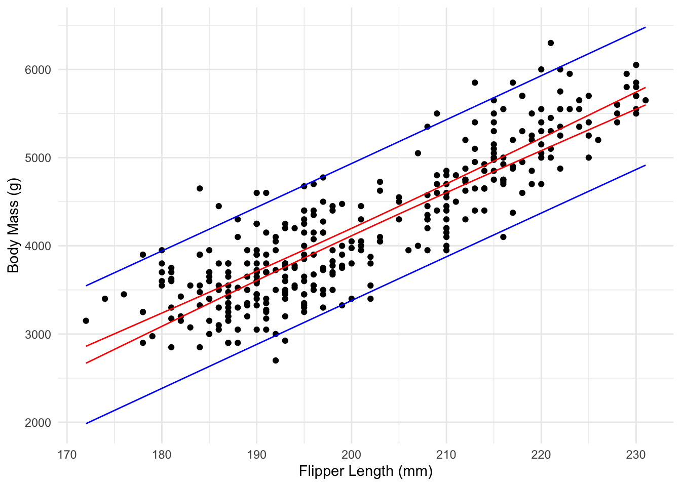
The following plot shows confidence and prediction intervals for the penguin data, showing the difference between them and how they change as \(x_{new}\) changes.
Computing these intervals in R
Thankfully, we rarely have to compute these quantities by hand. We can quickly get these from R as we fit a linear regression. We do this using the function predict for both prediction and confidence intervals.
Suppose we have a regression fit, which we think is reasonable.
penguin_fit <- lm(body_mass_g ~ flipper_length_mm, data = penguins)We can pass this as an argument to predict to get confidence and prediction intervals. We need to specify the new data point we want to predict at using a data.frame, with the same variable name as in the original data. We also need to specify whether we want a confidence interval (for the average value of \(y\)) or a prediction interval (for a new value of \(y\)) and the level of the interval.
new_x <- data.frame(flipper_length_mm = 200)

## to get a confidence interval
predict(penguin_fit, new_x, interval = "confidence", level = 0.95)
fit lwr upr
1 4156.282 4114.257 4198.307We can also get intervals for multiple points at once.
new_values <- data.frame(flipper_length_mm = c(150, 180,200, 220))

## to get a confidence interval
predict(penguin_fit, new_values, interval = "confidence", level = 0.95)
fit lwr upr
1 1672.004 1514.261 1829.746
2 3162.571 3087.333 3237.808
3 4156.282 4114.257 4198.307
4 5149.993 5079.229 5220.757The notation is almost identical for a prediction interval.
new_values <- data.frame(flipper_length_mm = c(150, 180,200, 220))

## to get a confidence interval
predict(penguin_fit, new_values, interval = "predict", level = 0.95)
fit lwr upr
1 1672.004 880.5922 2463.415
2 3162.571 2383.3979 3941.743
3 4156.282 3379.6125 4932.951
4 5149.993 4371.2398 5928.747Note that the prediction intervals are wider than confidence intervals for the same \(x\) at the same level. Note also that both intervals get wider the further we move away from \(\bar{x}\).
We can also construct confidence and prediction intervals if we have transformed the data. If we did a lof transformation of \(Y\) then our model is
\[ \log(Y) = \beta_0 + \beta_1 X + \epsilon, \]
so if we use predict it will give us an interval for \(\log(Y)\) rather than \(Y\). However, if we take the exponential of this interval, it is on the original scale of \(Y\). For example, if we fit a linear regression to \(\log(Y)\) of the species data we saw in class then we get a confidence interval for \(Y\) below.
       fit      lwr      upr
1 17.47610 12.01326 25.42308
2 17.52237 12.05122 25.47737
3 24.30548 17.25743 34.23199
2.9 Summary
Lets summarise what we have learned in this section by going through a complete example.
Example
Lets look at another dataset and go through the task of fitting a regression. Lets see if household income can be used to describe how much aid will be received by students going to a US college.
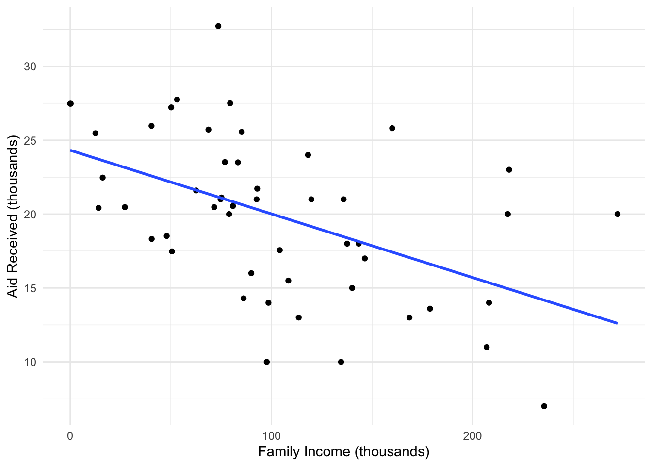
Here there appears to be a linear relationship, where as your family income increases you receive less aid. We need to check our regression first by looking at the residual plots we saw before.
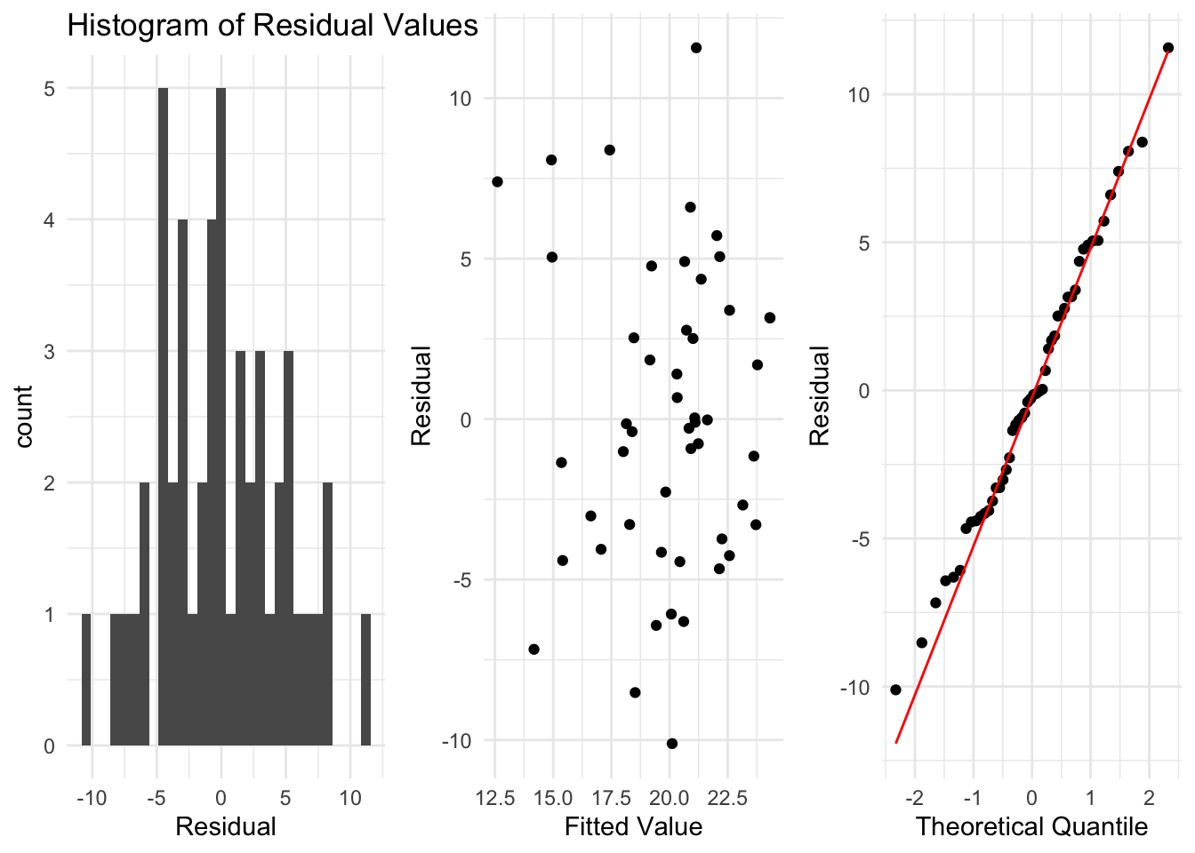
Looking at the residuals, we see no reasons to suspect the assumptions of linear regression are wrong, and so we can interpret the output of our model.
summary(elm_fit)
Call:
lm(formula = gift_aid ~ family_income, data = elmhurst)

Residuals:
     Min       1Q   Median       3Q      Max
-10.1128  -3.6234  -0.2161   3.1587  11.5707

Coefficients:
              Estimate Std. Error t value Pr(>|t|)
(Intercept)   24.31933    1.29145  18.831  < 2e-16 ***
family_income -0.04307    0.01081  -3.985 0.000229 ***
---
Signif. codes:  0 '***' 0.001 '**' 0.01 '*' 0.05 '.' 0.1 ' ' 1

Residual standard error: 4.783 on 48 degrees of freedom
Multiple R-squared:  0.2486,    Adjusted R-squared:  0.2329
F-statistic: 15.88 on 1 and 48 DF,  p-value: 0.0002289
For this example, we can actually interpret both coefficients. \(\hat{\beta}_0 = 24.32\), which says that if your family income is 0, you can expect to receive $24K in aid at this college. Similarly, \(\hat{\beta}_1 = -0.04\) means that, as your family income increases by 1000 dollars (here the \(x\) variable is in thousands), you can expect the aid you receive to decrease, on average, by $43.
Similarly, by looking at the output above, we see that both coefficients are statistically significantly different from 0.
Finally, we can use the regression model to construct a 95% confidence interval for how much aid the average student will receive, if their family income is 120k.
new_x <- data.frame(family_income = 120)

predict(elm_fit, new_x, interval = "confidence", level = 0.95)
fit lwr upr
1 19.15073 17.73432 20.56714Similarly, we can construct a 95% prediction interval, for how much aid a single student, with family income 80k, could receive.
new_x <- data.frame(family_income = 80)

predict(elm_fit, new_x, interval = "prediction", level = 0.95)
fit lwr upr
1 20.8736 11.15032 30.59687This section has provided a brief introduction to the ideas behind linear regression and shown how to fit a linear regression when you have one explanatory variable (\(x\)) and one dependent variable (\(y\)). We’ve learned how to assess whether a linear regression is suitable for data, how to fit a regression in R and how to interpret the regression fit, along with using it to understand the plausible values the coefficients (\(\beta_0,\beta_1\)) can take and how to predict the value of \(y\) at a new values of \(x\).
2.10 Practice Problems
Below are some additional practice problems related to this chapter. The solutions will be collapsed by default. Try to solve the problems on your own before looking at the solutions!
Problem 1
For a given dataset on shoulder girth and height of some individuals, the mean shoulder girth is 107.20 cm with a standard deviation of 10.37 cm. The mean height is 171.14 cm with a standard deviation of 9.41 cm. The correlation between height and shoulder girth is 0.67.
- Write the equation of the regression line for predicting height, making clear what \(x\) and \(y\) correspond to in the equation.
- Interpret the slope and intercept for this model (without computing them)
- Calculate \(R^2\) of the regression line for predicting height from shoulder girth, and interpret it in the context of the application
Solution
The equation for this regression model is \(y=\beta_0 +\beta_1 x + \epsilon\), where \(y\) is the height of the individual and \(x\) is the shoulder girth.
In this model, \(\beta_0\) is the average height of someone with shoulder girth of 0, which is not a sensible value to consider. \(\beta_1\) is the average in height (in cm) as shoulder girth increases by 1cm.
Here \(R^2 = .45\), which is a moderate value. This indicated some of the variability in height is captured by the relationship with shoulder girth, and shoulder girth explains about half of the variance in \(y\).
Problem 2
- Given that a linear regression model is appropriate for the data in Q1, compute \(\hat{\beta}_0\) and \(\hat{\beta}_1\)
- A randomly selected student has a shoulder girth of 100 cm. Predict the height of this student using the model estimated in the previous part
- The student from the previous part is 160 cm tall. Calculate the residual, and explain what this residual means
- A one year old has a shoulder girth of 56 cm. Would it be appropriate to use this linear model to predict the height of this child? Why/Why Not?
Solution
To compute these we have \(\hat{\beta}_1 = 0.67 \times \left(\frac{9.41}{10.37})\right) = 0.608\) and \(\hat{\beta}_0 = 171.14-0.608\times 107.20 = 1105.96\).
For \(x=100\) this gives \(\hat{y} = 105.96 + 0.608(100) = 166.76\).
The residual is \(e_i = y_i -\hat{y}_i = -6.76\), meaning the true \(y\) like 6.76 units below the fitted line.
Here \(56\)cm is very different to the mean of this sample, so its possible that this would be a large outlier. We would need to see if any data in that region currently, but may lead to extrapolation, meaning its not an appropriate model there.
Problem 3
The following data describes the grades 233 students received on a standardized test (exam1), along with their overall grades in a college course. The output from fitting this regression in R is shown.
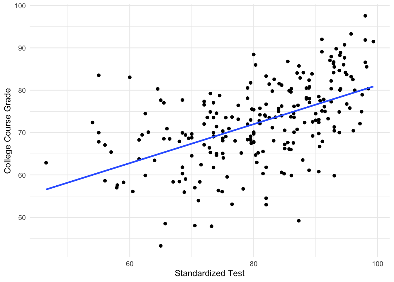
Call:
lm(formula = course_grade ~ exam1, data = data)

Residuals:
     Min       1Q   Median       3Q      Max
-26.1508  -4.6656   0.6166   5.6247  23.0312

Coefficients:
            Estimate Std. Error t value Pr(>|t|)
(Intercept) 35.17049    3.99911   8.795 3.44e-16 ***
exam1        0.46032    0.04906   9.383  < 2e-16 ***
---
Signif. codes:  0 '***' 0.001 '**' 0.01 '*' 0.05 '.' 0.1 ' ' 1

Residual standard error: 8.252 on 230 degrees of freedom
  (1 observation deleted due to missingness)
Multiple R-squared:  0.2768,    Adjusted R-squared:  0.2737
F-statistic: 88.04 on 1 and 230 DF,  p-value: < 2.2e-16
Given this output, and that a linear regression is a reasonable model for this data:
- Construct a 95% confidence interval for the slope coefficient
- Given this estimate, do you think it is reasonable to claim that the slope is zero?
- Does the intercept term have a natural interpretation for this data?
- Suppose a 95% confidence interval for the average Course Grade for a standardized test score of 70 is \((65.90, 68.88)\). How would this interval change if we instead looked at a prediction interval?
Solution
For this problem we have \(\hat{\beta}_1=0.46\) and \(se(\hat{\beta}_1)= 0.049\). We need to compute \(t_{230,0.025}=1.98\) which can be done with qt(0.025, df = 231, lower.tail = FALSE).
Then the interval will be \((\hat{\beta}_1 - 1.98 se(\hat{\beta}_1), \hat{\beta}_1 + 1.98 se(\hat{\beta}_1) = (0.36, 0.55).\)
As this confidence interval doesn’t contain zero, there is evidence to reject the null hypothesis that \(\beta_1=0\) at \(\alpha = 0.05\).
Here the intercept corresponds to the average grade a student would expect to get in this course if they got 0 on the standardized test. This might be plausible, for certain types of tests.
A prediction interval is always wider than a confidence interval due to the additional uncertainty. Therefore, the lower value would drecrease and the upper values would increase.
Problem 4
A researcher wants to examine the relationship between the grade a student receives in a class (\(y\)) and the hours of tv they watch in a week (\(x\)).
They fit a regression (shown below), along with plotting the residuals.
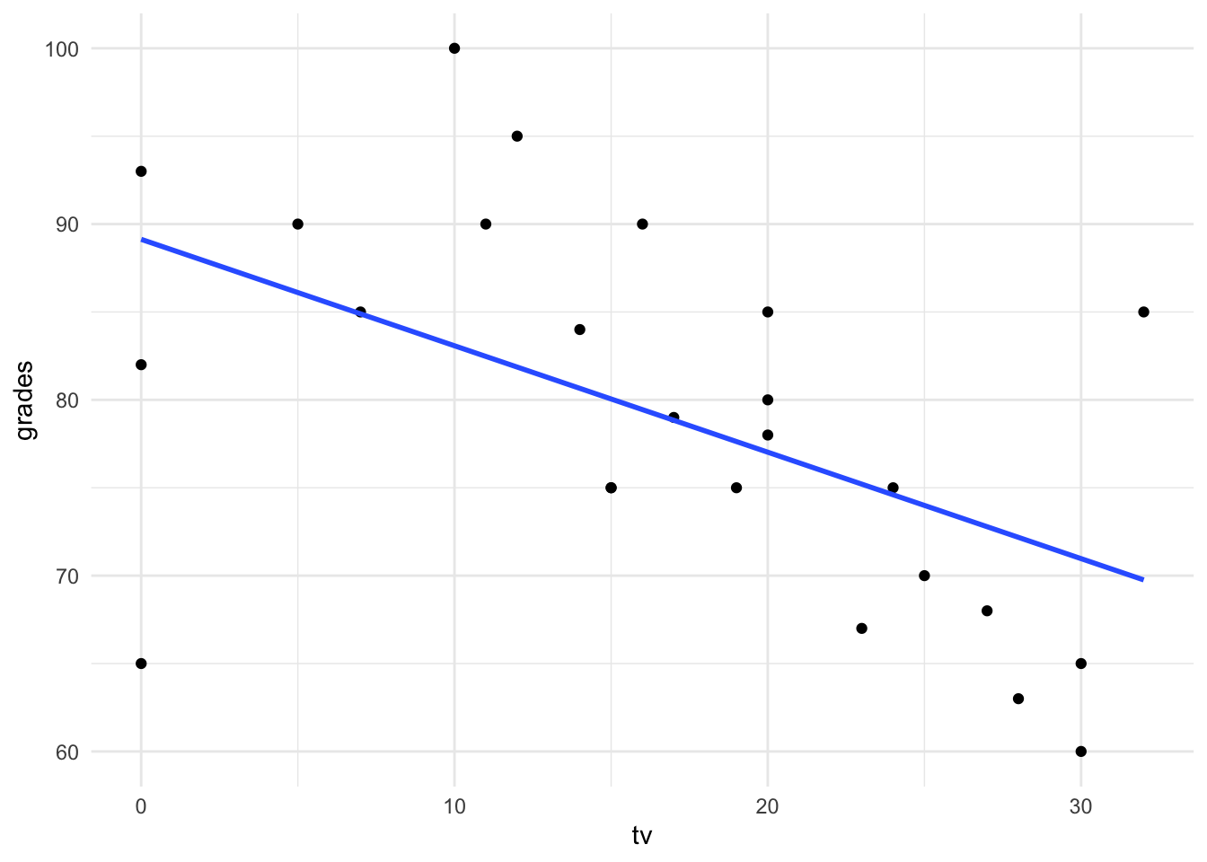
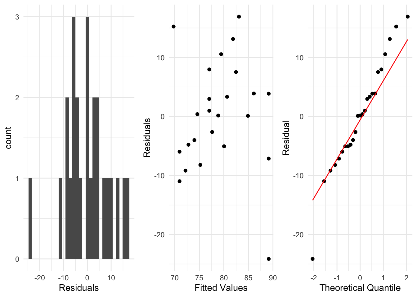
Pick one of the residual plots shown and describe how you use it to check whether the assumptions of a linear regression are satisfied.
Given these plots, do you see any potential issues with the regression for this data? How could they be addressed?
Solution
For the middle residual plot, we aim to check that there is no pattern in the residuals and the variance of the residuals doesn’t change from left to right in the plot.
From these plots, there are some residuals which indicate problems with the fitted regression model. These could be addressed by transforming the \(Y\) variable, using \(\log(Y)\) instead for example, and examining the residuals from that model.