ppdiag is an R package which provides a collection of tools which can be used to assess the fit of temporal point processes to data.
These currently include:
- Simulating data from a specified point process
- Fitting a specified point process model to data
- Evaluating the fit of a point process model to data using several diagnostic tools
Installation
You can install the released version of ppdiag from CRAN with:
install.packages("ppdiag")The current development version of this package is available from GitHub with:
# install.packages("remotes")
remotes::install_github("OwenWard/ppdiag")
Example
To illustrate some of the basic functionality of this package, we can simulate data from a specified Hawkes process and examine our diagnostic results when we fit a homogeneous Poisson process to this data.
library(ppdiag)

hp_obj <- pp_hp(lambda0 = 0.2, alpha = 0.35, beta = 0.8)
sim_hp <- pp_simulate(hp_obj, end = 200)
sim_hp
#>  [1]   5.760803   8.948532   9.985766  11.144890  11.305228  17.509538
#>  [7]  21.990103  25.754804  25.756725  26.663477  30.420693  34.465694
#> [13]  36.599366  41.410990  44.438180  44.712109  45.211409  46.512076
#> [19]  49.511806  51.046608  52.335976  75.660840  76.639780  85.685473
#> [25]  87.284500  87.448896  87.722795  87.856140  89.034916  89.056869
#> [31]  89.179466  89.195399  90.775515  90.792069  91.042053  92.293751
#> [37]  92.355206  96.928276  97.053098  97.880772  98.310011  98.881077
#> [43]  99.010649  99.213401  99.347277 100.022472 100.679788 100.694527
#> [49] 101.452972 103.926526 106.653150 113.212708 113.738940 114.338943
#> [55] 114.745921 115.058328 115.128879 115.896050 116.130131 116.241804
#> [61] 118.427450 123.380339 123.502200 123.973237 128.881506 129.263522
#> [67] 143.028509 151.006471 158.349391 162.063008 168.034982 170.657158
#> [73] 171.781831 175.347477 175.762528 176.398255 176.780393 182.373018
#> [79] 191.028275 191.257033 192.095983 196.416187 197.413321
We can readily evaluate the fit of a homogeneous Poisson process to this data.
est_hpp <- fithpp(sim_hp)
est_hpp
#> $lambda
#> [1] 0.4204377
#>
#> $events
#>  [1]   5.760803   8.948532   9.985766  11.144890  11.305228  17.509538
#>  [7]  21.990103  25.754804  25.756725  26.663477  30.420693  34.465694
#> [13]  36.599366  41.410990  44.438180  44.712109  45.211409  46.512076
#> [19]  49.511806  51.046608  52.335976  75.660840  76.639780  85.685473
#> [25]  87.284500  87.448896  87.722795  87.856140  89.034916  89.056869
#> [31]  89.179466  89.195399  90.775515  90.792069  91.042053  92.293751
#> [37]  92.355206  96.928276  97.053098  97.880772  98.310011  98.881077
#> [43]  99.010649  99.213401  99.347277 100.022472 100.679788 100.694527
#> [49] 101.452972 103.926526 106.653150 113.212708 113.738940 114.338943
#> [55] 114.745921 115.058328 115.128879 115.896050 116.130131 116.241804
#> [61] 118.427450 123.380339 123.502200 123.973237 128.881506 129.263522
#> [67] 143.028509 151.006471 158.349391 162.063008 168.034982 170.657158
#> [73] 171.781831 175.347477 175.762528 176.398255 176.780393 182.373018
#> [79] 191.028275 191.257033 192.095983 196.416187 197.413321
#>
#> attr(,"class")
#> [1] "hpp"

pp_diag(est_hpp, events = sim_hp)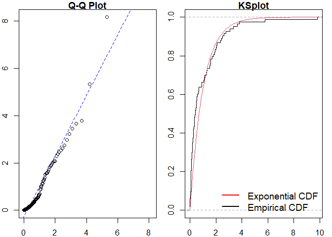
#>
#> Raw residual: 0
#> Pearson residual: -2.842171e-14
#>
#>  One-sample Kolmogorov-Smirnov test
#>
#> data:  r
#> D = 0.18659, p-value = 0.00529
#> alternative hypothesis: two-sided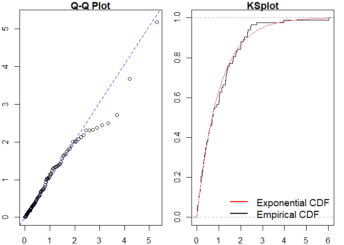
#> Raw residual: -0.005375166
#> Pearson residual: -0.3651356
#>
#>  One-sample Kolmogorov-Smirnov test
#>
#> data:  r
#> D = 0.064572, p-value = 0.8571
#> alternative hypothesis: two-sided
Markov Modulated Hawkes Process Example
This is particularly useful for more complex point processes, such as the Markov Modulated Hawkes Process (MMHP). We can simulate events from this model and examine the fit of simpler point processes to this data.
Q <- matrix(c(-0.2, 0.2, 0.1, -0.1), ncol = 2, byrow = TRUE)

mmhp_obj <- pp_mmhp(Q, delta = c(1 / 3, 2 / 3),
          lambda0 = 0.2,
          lambda1 = .75,
          alpha = 0.4,
          beta = 0.8)

mmhp_obj
#> $Q
#>      [,1] [,2]
#> [1,] -0.2  0.2
#> [2,]  0.1 -0.1
#>
#> $delta
#> [1] 0.3333333 0.6666667
#>
#> $events
#> NULL
#>
#> $lambda0
#> [1] 0.2
#>
#> $lambda1
#> [1] 0.75
#>
#> $alpha
#> [1] 0.4
#>
#> $beta
#> [1] 0.8
#>
#> attr(,"class")
#> [1] "mmhp"
mmhp_events <- pp_simulate(mmhp_obj, n = 50)
We can easily fit a homogeneous Poisson process and visualise the goodness of fit.
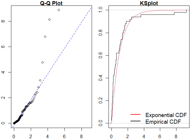
#>
#> Raw residual: -1
#> Pearson residual: -0.9740881
#>
#>  One-sample Kolmogorov-Smirnov test
#>
#> data:  r
#> D = 0.21168, p-value = 0.01914
#> alternative hypothesis: two-sided
Similarly for a Hawkes process.
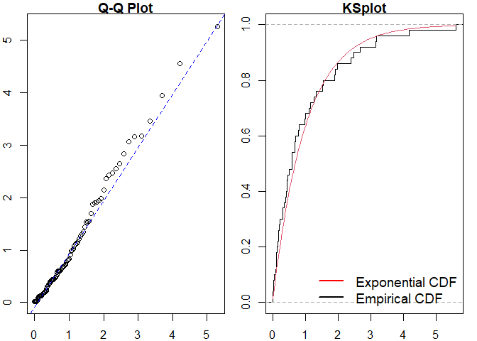
#> Raw residual: -0.3466309
#> Pearson residual: -0.6079909
#>
#>  One-sample Kolmogorov-Smirnov test
#>
#> data:  r
#> D = 0.095638, p-value = 0.7142
#> alternative hypothesis: two-sided
We can then compare to the true point process model.
pp_diag(mmhp_obj, mmhp_events$events)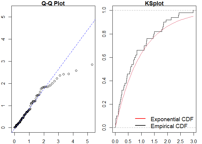
#> Raw residual: 8.862914
#> Pearson residual: 10.62449
#>
#>  One-sample Kolmogorov-Smirnov test
#>
#> data:  r
#> D = 0.096698, p-value = 0.7017
#> alternative hypothesis: two-sided
Getting help and contributing
Please file any issues here. Similarly, we would be delighted if anyone would like to contribute to this package (such as adding other point processes, kernel functions). Feel free to take a look here and reach out with any questions.
References
- Sun et al., (2021). ppdiag: Diagnostic Tools for Temporal Point Processes. Journal of Open Source Software, 6(61), 3133, https://doi.org/10.21105/joss.03133
- Wu et al., Diagnostics and Visualization of Point Process Models for Event Times on a Social Network, https://arxiv.org/abs/2001.09359
